鉴于深度学习出色的非线性表征能力,其被普遍用于进行从输入到给定标签数据集的输出的映射,即:图像分类,需要有人工标注标签的数据集.但是,不管是对 XRay 图像的标注,还是对新闻报道的主题的标注,都依赖于人工进行,尤其是针对大规模数据集,其工作量很大,费时费力.
聚类分析,也叫聚类(clustering),是一种无监督机器学习技术,其不需要带标注的标签数据集,只需根据数据样本的相似性对数据集进行分组.
聚类机器学习中,需要关注的技术,其原因如下.
1. 聚类的应用场景
[1] - 推荐系统
通过对用户购物记录的学习,聚类模型可以根据相似性对用户分组,以有助于寻找相似兴趣的用户,或用户感兴趣的相关产品.
[2] - 生物学中的序列聚类
序列聚类算法(sequence clustering) 生物序列根据相似性分组,其根据氨基酸(amino acid content) 含量对蛋白(proteins)进行聚类.
[3] - 图像或视频聚类分析
基于相似性将图像或视频进行聚类分析,以分组.
[4] - 医疗数据库中的应用
在医疗数据集场景中,每个病人可能包含不同的特定测试(如葡萄糖glucose,胆固醇cholesterol). 首先对病人进行聚类分析,有助于理解有价值的特征,以减少特征稀疏性;以及提升如癌症病人生存预测的分类任务上的准确性.
[5] - 通用场景
聚类可以得到数据的更紧凑汇总,以用于分类,模式发现,假设生成及测试.
对于数据科学家而言,聚类是非常有价值的.
2. 如何生成好的聚类
一个好的聚类方法应该生成高质量的聚类,其特点如:
[1] - 群组内部的高相似性:群组内的紧密聚合
High intra-class similarity: Cohesive within clusters
[2] - 群组之间的低相似性:群组之间各不相同
Low inter-class similarity: Distinctive between clusters
3. 采用 K-Means 设置 baseline
传统的 K-Means 算法具有较快的速度,并应用于各种问题. 然而,K-Means 算法的距离度量受限于原始数据空间. 对于输入数据的维度较高时,如图像数据,算法效率会较低.
以 MNIST 手写数据集为例,训练 K-Means 模型来进行聚类为 10 个组:
from sklearn.cluster import KMeans
from keras.datasets import mnist

(x_train, y_train), (x_test, y_test) = mnist.load_data()
x = np.concatenate((x_train, x_test))
y = np.concatenate((y_train, y_test))
x = x.reshape((x.shape[0], -1))
x = np.divide(x, 255.)
# 10 clusters
n_clusters = len(np.unique(y))
# Runs in parallel 4 CPUs
kmeans = KMeans(n_clusters=n_clusters, n_init=20, n_jobs=4)
# Train K-Means.
y_pred_kmeans = kmeans.fit_predict(x)
# Evaluate the K-Means clustering accuracy.
metrics.acc(y, y_pred_kmeans)
得到 K-Means 聚类算法的准确度为 53.2%. 后会将它与深度嵌入聚类模型(deep embedding clustering model)进行对比分析.
深度嵌入聚类模型主要包括:
[1] - 一个自动编码器,预训练,以学习无标签数据集的初始压缩后的特征表示.
[2] - 在编码器上堆积聚类层(clustering),以分配编码器输出到一个聚类组. 聚类层的权重初始化采用的是基于当前得到的 K-Means 聚类中心.
[3] - 聚类模型的训练,以同时改善聚类层和编码器.
Keras_Deep_Clustering
4. 预训练自编码器
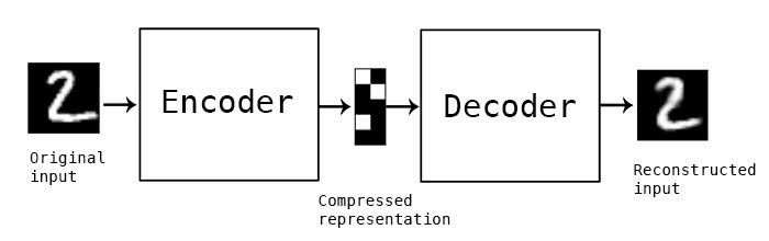
自动编码器是一种数据压缩算法,其主要包括编码器和解码器两个部分.
编码器将输入数据压缩为较低维度的特征. 如,一张 28x28 的 MNIST 图像总共有 784 个像素,编码器可以将其压缩为 10 个浮点数组成的数组. 这些浮点数称作图像的特征.
而解码器采用压缩后的特征作为输入,并尽可能的重建与原始图像尽可能相似的图像.
自动编码器是一中无监督学习算法,其训练只需要图像本身,而不需要标注标签.
自编码器
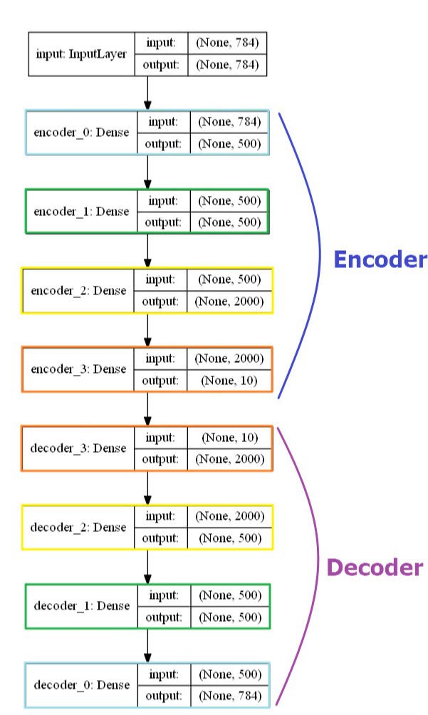
构建的自动编码器是一个全连接对称模型,其对称性在于,图像的压缩和解压过程是一组完全对应的相反过程.
全连接自编码器
训练自动编码器 300 个 epochs,并保存模型权重:
autoencoder.fit(x, x, batch_size=256, epochs=300) #, callbacks=cb)
autoencoder.save_weights('./results/ae_weights.h5')
5. 聚类模型
自动编码器训练后,其编码器部分将每幅图像压缩成 10 个浮点数. 对此,因为输入数据的维度降低到了 10,因此可以采用 K-Means 算法生成聚类中心,其是 10 维特征空间的 10 个聚类中心.
但,这里还构建了自定义的聚类层,以将输入特征转换为聚类标签概率.
聚类标签概率的计算采用的是 t-分布.
T-分布,与 t-SNE 算法中的应用一致,其度量了中心点和嵌入点之间的相似性.
自定义的模型聚类曾,类似于 K-Means 聚类,其权重表示聚类中心,其根据训练的 K-Means 进行初始化.
Keras 中创建自定义网络层,主要包括三种实现方法:
[1] - build(input_shape) - 定义网络层的权重,这里是 10-D 特征空间的 10 个聚类,即,10x10 个权重变量.
[2] - call(x) - 网络层逻辑定义,即,将特征映射到聚类标签.
[3] - compute_output_shape(input_shape) - 指定输入 shapes 到输出 shapes 的 shape 变换逻辑.
如:
class ClusteringLayer(Layer):
    """
    Clustering layer converts input sample (feature) to soft label.
    # Example
    model.add(ClusteringLayer(n_clusters=10))

    # Arguments
        n_clusters: number of clusters.
        weights: list of Numpy array with shape `(n_clusters, n_features)` witch represents the initial cluster centers.
        alpha: degrees of freedom parameter in Student's t-distribution. Default to 1.0.
    # Input shape
        2D tensor with shape: `(n_samples, n_features)`.
    # Output shape
        2D tensor with shape: `(n_samples, n_clusters)`.
    """

    def __init__(self, n_clusters, weights=None, alpha=1.0, **kwargs):
        if 'input_shape' not in kwargs and 'input_dim' in kwargs:
            kwargs['input_shape'] = (kwargs.pop('input_dim'),)
        super(ClusteringLayer, self).__init__(**kwargs)
        self.n_clusters = n_clusters
        self.alpha = alpha
        self.initial_weights = weights
        self.input_spec = InputSpec(ndim=2)

    def build(self, input_shape):
        assert len(input_shape) == 2
        input_dim = input_shape[1]
        self.input_spec = InputSpec(dtype=K.floatx(), shape=(None, input_dim))
        self.clusters = self.add_weight((self.n_clusters, input_dim),
                                        initializer='glorot_uniform',
                                        name='clusters')
        if self.initial_weights is not None:
            self.set_weights(self.initial_weights)
            del self.initial_weights
        self.built = True

    def call(self, inputs, **kwargs):
        """ student t-distribution, as same as used in t-SNE algorithm.
                 q_ij = 1/(1+dist(x_i, µ_j)^2), then normalize it.
                 q_ij can be interpreted as the probability of assigning sample i to cluster j.
                 (i.e., a soft assignment)
        Arguments:
            inputs: the variable containing data, shape=(n_samples, n_features)
        Return:
            q: student's t-distribution, or soft labels for each sample. shape=(n_samples, n_clusters)
        """
        q = 1.0 / (1.0 + (K.sum(K.square(K.expand_dims(inputs, axis=1) - self.clusters), axis=2) / self.alpha))
        q **= (self.alpha + 1.0) / 2.0
        q = K.transpose(K.transpose(q) / K.sum(q, axis=1)) # Make sure each sample's 10 values add up to 1.
        return q

    def compute_output_shape(self, input_shape):
        assert input_shape and len(input_shape) == 2
        return input_shape[0], self.n_clusters

    def get_config(self):
        config = {'n_clusters': self.n_clusters}
        base_config = super(ClusteringLayer, self).get_config()
        return dict(list(base_config.items()) + list(config.items()))
然后,预训练的编码器后堆叠聚类层,以形成聚类模型.
对于聚类层,采用 K-Means 对所有图像的特征向量进行训练,得到的聚类中心初始化聚类层权重.
clustering_layer = ClusteringLayer(n_clusters, name='clustering')(encoder.output)
model = Model(inputs=encoder.input, outputs=clustering_layer)
# Initialize cluster centers using k-means.
kmeans = KMeans(n_clusters=n_clusters, n_init=20)
y_pred = kmeans.fit_predict(encoder.predict(x))
model.get_layer(name='clustering').set_weights([kmeans.cluster_centers_])
聚类模型结构
6. 训练聚类模型
6.1. 辅助目标分布和 KL 散度损失
(Auxiliary target distribution and KL divergence loss)
接着要做的是,同时提升聚类和特征表示的效果.
为此,将定义一个基于质心的目标概率分布( centroid-based target probability distribution),并根据模型聚类结果最小化 KL 散度.
目标分布应该具有以下属性:
[1] - 加强预测,如,提升聚类精度.
Strengthen predictions, i.e., improve cluster purity.
[2] - 更关注于高置信度的数据样本.
Put more emphasis on data points assigned with high confidence.
[3] - 避免大聚类组干扰隐藏特征空间.
Prevent large clusters from distorting the hidden feature space.
目标分布的计算,首先将 q(编码的特征向量) 提升到第二幂(second power),然后,根据每个聚类组的频率进行归一化.(The target distribution is computed by first raising q (the encoded feature vectors) to the second power and then normalizing by frequency per cluster.)
def target_distribution(q):
    weight = q ** 2 / q.sum(0)
    return (weight.T / weight.sum(1)).T
有必要基于辅助目标分布的帮助,以从高置信度的结果中进行学习,进而迭代的改善聚类结果. 进行特征次数的迭代后,目标分布得到了更新,待训练聚类模型最小化目标分布和聚类输出间的 KL 散度损失函数. 训练策略可以看作自训练(self-training) 的一种形式. 类似于自训练,采用初始化分类器和无标签数据集,然后根据分类器标记数据集,以在其高置信度预测结果上进行训练.
损失函数,KL散度(Kullback-Leibler散度),衡量了两种不同分布之间的差异性. 对其进行最小化,使得目标分布尽可能接近聚类输出分布.
如下面的代码段,每 140 个 epochs 训练迭代,更新目标分布:
model.compile(optimizer=SGD(0.01, 0.9), loss='kld')

maxiter = 8000
update_interval = 140
for ite in range(int(maxiter)):
    if ite % update_interval == 0:
        q = model.predict(x, verbose=0)
        # update the auxiliary target distribution p
        p = target_distribution(q)
        # evaluate the clustering performance
        y_pred = q.argmax(1)
        if y is not None:
            acc = np.round(metrics.acc(y, y_pred), 5)

    idx = index_array[index * batch_size: min((index+1) * batch_size, x.shape[0])]
    model.train_on_batch(x=x[idx], y=p[idx])
    index = index + 1 if (index + 1) * batch_size <= x.shape[0] else 0
每次更新后,可以看出,聚类准确度在稳步提升.
6.2. 评价度量
评价度量表明,已达到 96.2% 的聚类精度. 对于输入是未标记的图像,这个结果很不错了. 对该聚类精度分析.
该度量找出无监督算法的聚类和 groundtruth 间的最佳匹配.
可以采用 Hungarian 算法 有效的得到该最佳映射,其实现如:scikit learn 库的 linear_assignment 函数.
from sklearn.utils.linear_assignment_ import linear_assignment

y_true = y.astype(np.int64)
D = max(y_pred.max(), y_true.max()) + 1
w = np.zeros((D, D), dtype=np.int64)
# Confusion matrix.
for i in range(y_pred.size):
    w[y_pred[i], y_true[i]] += 1
ind = linear_assignment(-w)
acc = sum([w[i, j] for i, j in ind]) * 1.0 / y_pred.size
更直接的可视化 - 混淆矩阵:
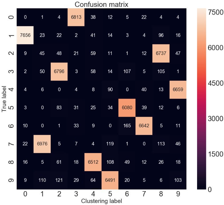
混淆矩阵
可以手动快速匹配聚类,如,聚类 1与真实标签 7 或手写数字7相匹配.
混淆矩阵的实现:
import seaborn as sns
import sklearn.metrics
import matplotlib.pyplot as plt
sns.set(font_scale=3)
confusion_matrix = sklearn.metrics.confusion_matrix(y, y_pred)

plt.figure(figsize=(16, 14))
sns.heatmap(confusion_matrix, annot=True, fmt="d", annot_kws={"size": 20});
plt.title("Confusion matrix", fontsize=30)
plt.ylabel('True label', fontsize=25)
plt.xlabel('Clustering label', fontsize=25)
plt.show()
7. 卷积自编码
针对图像数据集,可以尝试卷积自动编码器,而不是仅使用全连接层.
值得说的是,为了重建图像,可以采用 deconvolutional 层 (Conv2DTranspose in Keras) 或上采样层(UpSampling2D) 以减少 artifacts 问题.
8.总结及阅读材料
这里介绍了基于 Keras 模型进行无监督聚类分析的方法. 预训练的自编码器对于降维和参数初始化具有重要作用,然后自定义聚类层,其对目标分布进行训练,以进一步改善精度.
9. 完整实现
Keras-DEC.ipynb
import numpy as np
np.random.seed(10)

from time import time
import keras.backend as K
from keras.engine.topology import Layer, InputSpec
from keras.layers import Dense, Input
from keras.models import Model
from keras.optimizers import SGD
from keras import callbacks
from keras.initializers import VarianceScaling
from keras.datasets import mnist
from sklearn.cluster import KMeans
import metrics
9.1. 定义自编码器
# 定义自编码器模型
def autoencoder(dims, act='relu', init='glorot_uniform'):
    """
    全连接自编码模型,对称结构.
    Arguments:
        dims: list of number of units in each layer of encoder.
              dims[0] is input dim, dims[-1] is units in hidden layer.
              The decoder is symmetric with encoder.
              So number of layers of the auto-encoder is 2*len(dims)-1
        act: activation, not applied to Input, Hidden and Output layers
    return:
        (ae_model, encoder_model), Model of autoencoder and model of encoder
    """
    n_stacks = len(dims) - 1
    # input
    input_img = Input(shape=(dims[0],), name='input')
    x = input_img
    # internal layers in encoder
    for i in range(n_stacks-1):
        x = Dense(dims[i + 1],
                  activation=act,
                  kernel_initializer=init,
                  name='encoder_%d' % i)(x)

    # hidden layer,features are extracted from here
    encoded = Dense(dims[-1],
                    kernel_initializer=init,
                    name='encoder_%d' % (n_stacks - 1))(x)

    x = encoded
    # internal layers in decoder
    for i in range(n_stacks-1, 0, -1):
        x = Dense(dims[i],
                  activation=act,
                  kernel_initializer=init,
                  name='decoder_%d' % i)(x)

    # output
    x = Dense(dims[0], kernel_initializer=init, name='decoder_0')(x)
    decoded = x

    return Model(inputs=input_img, outputs=decoded, name='AE'),
           Model(inputs=input_img, outputs=encoded, name='encoder')
9.2. 加载数据
(x_train, y_train), (x_test, y_test) = mnist.load_data()

x = np.concatenate((x_train, x_test))
y = np.concatenate((y_train, y_test))
x = x.reshape((x.shape[0], -1))
x = np.divide(x, 255.)
n_clusters = len(np.unique(y))
# x.shape:(70000, 784)
9.3. K-Means 聚类精度 baseline
# 定义精度函数
from sklearn.metrics import normalized_mutual_info_score, adjusted_rand_score
from sklearn.utils.linear_assignment_ import linear_assignment

nmi = normalized_mutual_info_score
ari = adjusted_rand_score

def acc(y_true, y_pred):
    """
    Calculate clustering accuracy. Require scikit-learn installed
    # Arguments
        y: true labels, numpy.array with shape `(n_samples,)`
        y_pred: predicted labels, numpy.array with shape `(n_samples,)`
    # Return
        accuracy, in [0,1]
    """
    y_true = y_true.astype(np.int64)
    assert y_pred.size == y_true.size
    D = max(y_pred.max(), y_true.max()) + 1
    w = np.zeros((D, D), dtype=np.int64)
    for i in range(y_pred.size):
        w[y_pred[i], y_true[i]] += 1

    ind = linear_assignment(w.max() - w)
    return sum([w[i, j] for i, j in ind]) * 1.0 / y_pred.size


kmeans = KMeans(n_clusters=n_clusters, n_init=20, n_jobs=4)
y_pred_kmeans = kmeans.fit_predict(x)

acc_baseline = acc(y, y_pred_kmeans)
# 0.5322857142857143
9.4. 自编码器训练
dims = [x.shape[-1], 500, 500, 2000, 10]
init = VarianceScaling(scale=1. / 3.,
                       mode='fan_in',
                       distribution='uniform')
pretrain_optimizer = SGD(lr=1, momentum=0.9)
pretrain_epochs = 300
batch_size = 256
save_dir = './results'

autoencoder, encoder = autoencoder(dims, init=init)
9.4.1. 自编码器可视化
from keras.utils import plot_model
plot_model(autoencoder, to_file='autoencoder.png', show_shapes=True)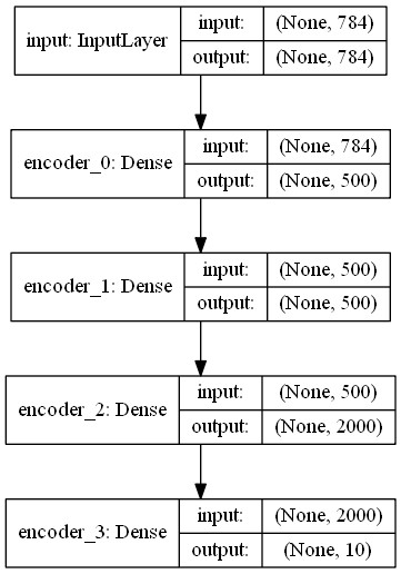
9.4.2. 编码器可视化
from keras.utils import plot_model
plot_model(encoder, to_file='encoder.png', show_shapes=True)
9.4.3. 自编码器预训练
autoencoder.compile(optimizer=pretrain_optimizer, loss='mse')
autoencoder.fit(x, x, batch_size=batch_size, epochs=pretrain_epochs) #, callbacks=cb)
autoencoder.save_weights(save_dir + '/ae_weights.h5')
# autoencoder.load_weights(save_dir + '/ae_weights.h5')
训练过程:
Epoch 1/300
70000/70000 [==============================] - 4s 59us/step - loss: 0.0647
Epoch 2/300
70000/70000 [==============================] - 2s 35us/step - loss: 0.0424
Epoch 3/300
70000/70000 [==============================] - 2s 35us/step - loss: 0.0310
Epoch 4/300
70000/70000 [==============================] - 2s 35us/step - loss: 0.0261
Epoch 5/300
70000/70000 [==============================] - 2s 35us/step - loss: 0.0238
Epoch 6/300
70000/70000 [==============================] - 2s 35us/step - loss: 0.0223
Epoch 7/300
70000/70000 [==============================] - 2s 35us/step - loss: 0.0211
...
Epoch 298/300
70000/70000 [==============================] - 2s 34us/step - loss: 0.0083
Epoch 299/300
70000/70000 [==============================] - 2s 35us/step - loss: 0.0083
Epoch 300/300
70000/70000 [==============================] - 2s 35us/step - loss: 0.0083
9.5. 构建聚类模型
9.5.1. ClusteringLayer 自定义聚类层
class ClusteringLayer(Layer):
    """
    聚类层,将输入样本(特征)转换为 soft label,
    如,表示了每个样本属于每个聚类的概率向量.
    概率时根据 student's t-distribution 计算得到.

    # Example
    model.add(ClusteringLayer(n_clusters=10))

    # Arguments
        n_clusters: number of clusters.
        weights: list of Numpy array with shape `(n_clusters, n_features)` which represents the initial cluster centers.
        alpha: degrees of freedom parameter in Student's t-distribution. Default to 1.0.
    # Input shape
        2D tensor with shape: `(n_samples, n_features)`.
    # Output shape
        2D tensor with shape: `(n_samples, n_clusters)`.
    """

    def __init__(self, n_clusters, weights=None, alpha=1.0, **kwargs):
        if 'input_shape' not in kwargs and 'input_dim' in kwargs:
            kwargs['input_shape'] = (kwargs.pop('input_dim'),)
        super(ClusteringLayer, self).__init__(**kwargs)
        self.n_clusters = n_clusters
        self.alpha = alpha
        self.initial_weights = weights
        self.input_spec = InputSpec(ndim=2)

    def build(self, input_shape):
        assert len(input_shape) == 2
        input_dim = input_shape[1]
        self.input_spec = InputSpec(dtype=K.floatx(), shape=(None, input_dim))
        self.clusters = self.add_weight((self.n_clusters, input_dim),
                                        initializer='glorot_uniform',
                                        name='clusters')
        if self.initial_weights is not None:
            self.set_weights(self.initial_weights)
            del self.initial_weights
        self.built = True

    def call(self, inputs, **kwargs):
        """
        student t-distribution,与 t-SNE 算法中的一致.
        度量了嵌入点 z_i 与中心点 µ_j 之间的 相似性.
        q_ij = 1/(1+dist(x_i, µ_j)^2), then normalize it.
        q_ij can be interpreted as the probability of assigning sample i to cluster j.
            (i.e., a soft assignment)
        Arguments:
            inputs: the variable containing data, shape=(n_samples, n_features)
        Return:
            q: student's t-distribution, or soft labels for each sample.
               shape=(n_samples, n_clusters)
        """
        q = 1.0 / (1.0 + (K.sum(K.square(K.expand_dims(inputs, axis=1) - self.clusters), axis=2) / self.alpha))
        q **= (self.alpha + 1.0) / 2.0

        # Make sure each sample's 10 values add up to 1.
        q = K.transpose(K.transpose(q) / K.sum(q, axis=1))
        return q

    def compute_output_shape(self, input_shape):
        assert input_shape and len(input_shape) == 2
        return input_shape[0], self.n_clusters

    def get_config(self):
        config = {'n_clusters': self.n_clusters}
        base_config = super(ClusteringLayer, self).get_config()
        return dict(list(base_config.items()) + list(config.items()))

clustering_layer = ClusteringLayer(n_clusters, name='clustering')(encoder.output)
model = Model(inputs=encoder.input, outputs=clustering_layer)

#模型可视化
from keras.utils import plot_model
plot_model(model, to_file='model.png', show_shapes=True)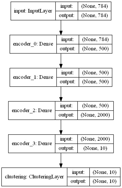
9.5.2. 聚类模型训练
model.compile(optimizer=SGD(0.01, 0.9), loss='kld')

# Step 1: 采用 K-Means 初始化聚类中心.
kmeans = KMeans(n_clusters=n_clusters, n_init=20)
y_pred = kmeans.fit_predict(encoder.predict(x))
y_pred_last = np.copy(y_pred)
model.get_layer(name='clustering').set_weights([kmeans.cluster_centers_])

# Step 2: 深度聚类(deep clustering)
# Compute p_i by first raising q_i to the second power and
# then normalizing by frequency per cluster:

# computing an auxiliary target distribution
def target_distribution(q):
    weight = q ** 2 / q.sum(0)
    return (weight.T / weight.sum(1)).T

loss = 0
index = 0
maxiter = 8000
update_interval = 140
index_array = np.arange(x.shape[0])
tol = 0.001 # tolerance threshold to stop training

# 开始训练
for ite in range(int(maxiter)):
    if ite % update_interval == 0:
        q = model.predict(x, verbose=0)

        # update the auxiliary target distribution p
        p = target_distribution(q)

        # evaluate the clustering performance
        y_pred = q.argmax(1)
        if y is not None:
            acc_ = np.round(acc(y, y_pred), 5)
            nmi_ = np.round(nmi(y, y_pred), 5)
            ari_ = np.round(ari(y, y_pred), 5)
            loss = np.round(loss, 5)
            print('Iter %d: acc = %.5f, nmi = %.5f, ari = %.5f' % (ite, acc_, nmi_, ari_), ' ; loss=', loss)

        # check stop criterion - model convergence
        delta_label = np.sum(y_pred != y_pred_last).astype(np.float32) / y_pred.shape[0]
        y_pred_last = np.copy(y_pred)
        if ite > 0 and delta_label < tol:
            print('delta_label ', delta_label, '< tol ', tol)
            print('Reached tolerance threshold. Stopping training.')
            break
    idx = index_array[index * batch_size: min((index+1) * batch_size, x.shape[0])]
    loss = model.train_on_batch(x=x[idx], y=p[idx])
    index = index + 1 if (index + 1) * batch_size <= x.shape[0] else 0

model.save_weights(save_dir + '/DEC_model_final.h5')

# Load the clustering model trained weights
# model.load_weights(save_dir + '/DEC_model_final.h5')

# Final Evaluation
# Eval.
q = model.predict(x, verbose=0)
p = target_distribution(q)  # update the auxiliary target distribution p

# 评估聚类精度
y_pred = q.argmax(1)
if y is not None:
    acc_ = np.round(acc(y, y_pred), 5)
    nmi_ = np.round(nmi(y, y_pred), 5)
    ari_ = np.round(ari(y, y_pred), 5)
    loss = np.round(loss, 5)
    print('Iter %d: acc = %.5f, nmi = %.5f, ari = %.5f' % (ite, acc_, nmi_, ari_), ' ; loss=', loss)
# Acc = 0.96231, nmi = 0.90500, ari = 0.91897  ; loss= 0
9.5.3. 混淆矩阵
import seaborn as sns
import sklearn.metrics
import matplotlib.pyplot as plt
sns.set(font_scale=3)
confusion_matrix = sklearn.metrics.confusion_matrix(y, y_pred)

plt.figure(figsize=(16, 14))
sns.heatmap(confusion_matrix, annot=True, fmt="d", annot_kws={"size": 20});
plt.title("Confusion matrix", fontsize=30)
plt.ylabel('True label', fontsize=25)
plt.xlabel('Clustering label', fontsize=25)
plt.show()
9.6. 卷积自编码器
Convolutional auto encoder.
from keras.models import Model
from keras import backend as K
from keras import layers
from keras.layers import Input, Dense,
            Conv2D, MaxPooling2D, UpSampling2D,
            Flatten, Reshape, Conv2DTranspose
from keras.models import Model
import numpy as np
9.6.1. 采用 Conv2DTranspose 重建图像
采用 Conv2DTranspose 重建图像.
def autoencoderConv2D_1(input_shape=(28, 28, 1),
                        filters=[32, 64, 128, 10]):
    input_img = Input(shape=input_shape)
    if input_shape[0] % 8 == 0:
        pad3 = 'same'
    else:
        pad3 = 'valid'
    x = Conv2D(filters[0],
               5,
               strides=2,
               padding='same',
               activation='relu',
               name='conv1',
               input_shape=input_shape)(input_img)

    x = Conv2D(filters[1],
               5,
               strides=2,
               padding='same',
               activation='relu',
               name='conv2')(x)

    x = Conv2D(filters[2],
               3,
               strides=2,
               padding=pad3,
               activation='relu',
               name='conv3')(x)

    x = Flatten()(x)
    encoded = Dense(units=filters[3], name='embedding')(x)
    x = Dense(
        units=filters[2]*int(input_shape[0]/8)*int(input_shape[0]/8),
        activation='relu')(encoded)

    x = Reshape(
        (int(input_shape[0]/8),
         int(input_shape[0]/8),
         filters[2]))(x)
    x = Conv2DTranspose(filters[1],
                        3,
                        strides=2,
                        padding=pad3,
                        activation='relu',
                        name='deconv3')(x)

    x = Conv2DTranspose(filters[0],
                        5,
                        strides=2,
                        padding='same',
                        activation='relu',
                        name='deconv2')(x)

    decoded = Conv2DTranspose(input_shape[2],
                              5,
                              strides=2,
                              padding='same',
                              name='deconv1')(x)
    return Model(inputs=input_img,
                 outputs=decoded,
                 name='AE'),
           Model(inputs=input_img,
                 outputs=encoded,
                 name='encoder')
9.6.2. 采用 UpSampling2D 重建图像
采用 UpSampling2D 重建图像.
def autoencoderConv2D_2(img_shape=(28, 28, 1)):
    """
    Conv2D auto-encoder model.
    Arguments:
        img_shape: e.g. (28, 28, 1) for MNIST
    return:
        (autoencoder, encoder),
        Model of autoencoder and model of encoder
    """
    input_img = Input(shape=img_shape)
    # Encoder
    x = Conv2D(16,
               (3, 3),
               activation='relu',
               padding='same',
               strides=(2, 2))(input_img)
    x = Conv2D(8,
               (3, 3),
               activation='relu',
               padding='same',
               strides=(2, 2))(x)
    x = Conv2D(8,
               (3, 3),
               activation='relu',
               padding='same',
               strides=(2, 2))(x)
    shape_before_flattening = K.int_shape(x)
    # at this point the representation is (4, 4, 8) i.e. 128-dimensional
    x = Flatten()(x)
    encoded = Dense(10, activation='relu', name='encoded')(x)

    # Decoder
    x = Dense(np.prod(shape_before_flattening[1:]),
              activation='relu')(encoded)
    # Reshape into an image of the same shape as before our last `Flatten` layer
    x = Reshape(shape_before_flattening[1:])(x)

    x = Conv2D(8, (3, 3), activation='relu', padding='same')(x)
    x = UpSampling2D((2, 2))(x)
    x = Conv2D(8, (3, 3), activation='relu', padding='same')(x)
    x = UpSampling2D((2, 2))(x)
    x = Conv2D(16, (3, 3), activation='relu')(x)
    x = UpSampling2D((2, 2))(x)
    decoded = Conv2D(1, (3, 3), activation='sigmoid', padding='same')(x)

    return Model(inputs=input_img,
                 outputs=decoded,
                 name='AE'),
           Model(inputs=input_img,
                 outputs=encoded,
                 name='encoder')
9.6.3. 以 Conv2DTranspose 为例
autoencoder, encoder = autoencoderConv2D_1()
autoencoder.summary()
如:
_________________________________________________________________
Layer (type)                 Output Shape              Param #
=================================================================
input_1 (InputLayer)         (None, 28, 28, 1)         0
_________________________________________________________________
conv1 (Conv2D)               (None, 14, 14, 32)        832
_________________________________________________________________
conv2 (Conv2D)               (None, 7, 7, 64)          51264
_________________________________________________________________
conv3 (Conv2D)               (None, 3, 3, 128)         73856
_________________________________________________________________
flatten_1 (Flatten)          (None, 1152)              0
_________________________________________________________________
embedding (Dense)            (None, 10)                11530
_________________________________________________________________
dense_1 (Dense)              (None, 1152)              12672
_________________________________________________________________
reshape_1 (Reshape)          (None, 3, 3, 128)         0
_________________________________________________________________
deconv3 (Conv2DTranspose)    (None, 7, 7, 64)          73792
_________________________________________________________________
deconv2 (Conv2DTranspose)    (None, 14, 14, 32)        51232
_________________________________________________________________
deconv1 (Conv2DTranspose)    (None, 28, 28, 1)         801
=================================================================
Total params: 275,979
Trainable params: 275,979
Non-trainable params: 0
_________________________________________________________________
9.6.4. 以 MNIST 数据集为例
from keras.datasets import mnist

# 加载数据集
(x_train, y_train), (x_test, y_test) = mnist.load_data()

x = np.concatenate((x_train, x_test))
y = np.concatenate((y_train, y_test))
x = x.reshape(x.shape + (1,))
x = np.divide(x, 255.)

# 预训练卷积自编码器模型
pretrain_epochs = 100
batch_size = 256
autoencoder.compile(optimizer='adadelta', loss='mse')
autoencoder.fit(x, x, batch_size=batch_size, epochs=pretrain_epochs)
autoencoder.save_weights(save_dir+'/conv_ae_weights.h5')
# autoencoder.load_weights(save_dir+'/conv_ae_weights.h5')
训练过程,如:
Epoch 1/100
70000/70000 [==============================] - 8s 108us/step - loss: 0.0797
Epoch 2/100
70000/70000 [==============================] - 5s 70us/step - loss: 0.0622
Epoch 3/100
70000/70000 [==============================] - 5s 70us/step - loss: 0.0482
Epoch 4/100
70000/70000 [==============================] - 5s 71us/step - loss: 0.0377
Epoch 5/100
70000/70000 [==============================] - 5s 69us/step - loss: 0.0325
...
Epoch 98/100
70000/70000 [==============================] - 5s 70us/step - loss: 0.0134
Epoch 99/100
70000/70000 [==============================] - 5s 69us/step - loss: 0.0134
Epoch 100/100
70000/70000 [==============================] - 5s 69us/step - loss: 0.0133
9.7. 构建基于卷积自编码器的聚类模型
clustering_layer = ClusteringLayer(n_clusters, name='clustering')(encoder.output)
model = Model(inputs=encoder.input, outputs=clustering_layer)
model.compile(optimizer='adam', loss='kld')

# Step 1: 采用 K-Means 初始化聚类中心.
kmeans = KMeans(n_clusters=n_clusters, n_init=20)
y_pred = kmeans.fit_predict(encoder.predict(x))
y_pred_last = np.copy(y_pred)
model.get_layer(name='clustering').set_weights([kmeans.cluster_centers_])

# Step 2: 深度聚类(deep clustering)
9.7.1. 聚类模型训练
loss = 0
index = 0
maxiter = 8000
update_interval = 140
index_array = np.arange(x.shape[0])
tol = 0.001 # tolerance threshold to stop training
# 开始训练
for ite in range(int(maxiter)):
if ite % update_interval == 0:
q = model.predict(x, verbose=0)
p = target_distribution(q) # update the auxiliary target distribution p
# evaluate the clustering performance
y_pred = q.argmax(1)
if y is not None:
acc_ = np.round(acc(y, y_pred), 5)
nmi_ = np.round(nmi(y, y_pred), 5)
ari_ = np.round(ari(y, y_pred), 5)
loss = np.round(loss, 5)
print('Iter %d: acc = %.5f, nmi = %.5f, ari = %.5f' % (ite, acc_, nmi_, ari_), ' ; loss=', loss)
# check stop criterion
delta_label = np.sum(y_pred != y_pred_last).astype(np.float32) / y_pred.shape[0]
y_pred_last = np.copy(y_pred)
if ite > 0 and delta_label < tol:
print('delta_label ', delta_label, '< tol ', tol)
print('Reached tolerance threshold. Stopping training.')
break
idx = index_array[index * batch_size: min((index+1) * batch_size, x.shape[0])]
loss = model.train_on_batch(x=x[idx], y=p[idx])
index = index + 1 if (index + 1) * batch_size <= x.shape[0] else 0
model.save_weights(save_dir + '/conv_DEC_model_final.h5')
# model.load_weights(save_dir + '/conv_DEC_model_final.h5')
# Final Evaluation
q = model.predict(x, verbose=0)
p = target_distribution(q) # update the auxiliary target distribution p
# evaluate the clustering performance
y_pred = q.argmax(1)
if y is not None:
acc_ = np.round(acc(y, y_pred), 5)
nmi_ = np.round(nmi(y, y_pred), 5)
ari_ = np.round(ari(y, y_pred), 5)
loss = np.round(loss, 5)
print('Acc = %.5f, nmi = %.5f, ari = %.5f' % (acc_, nmi_, ari_), ' ; loss=', loss)
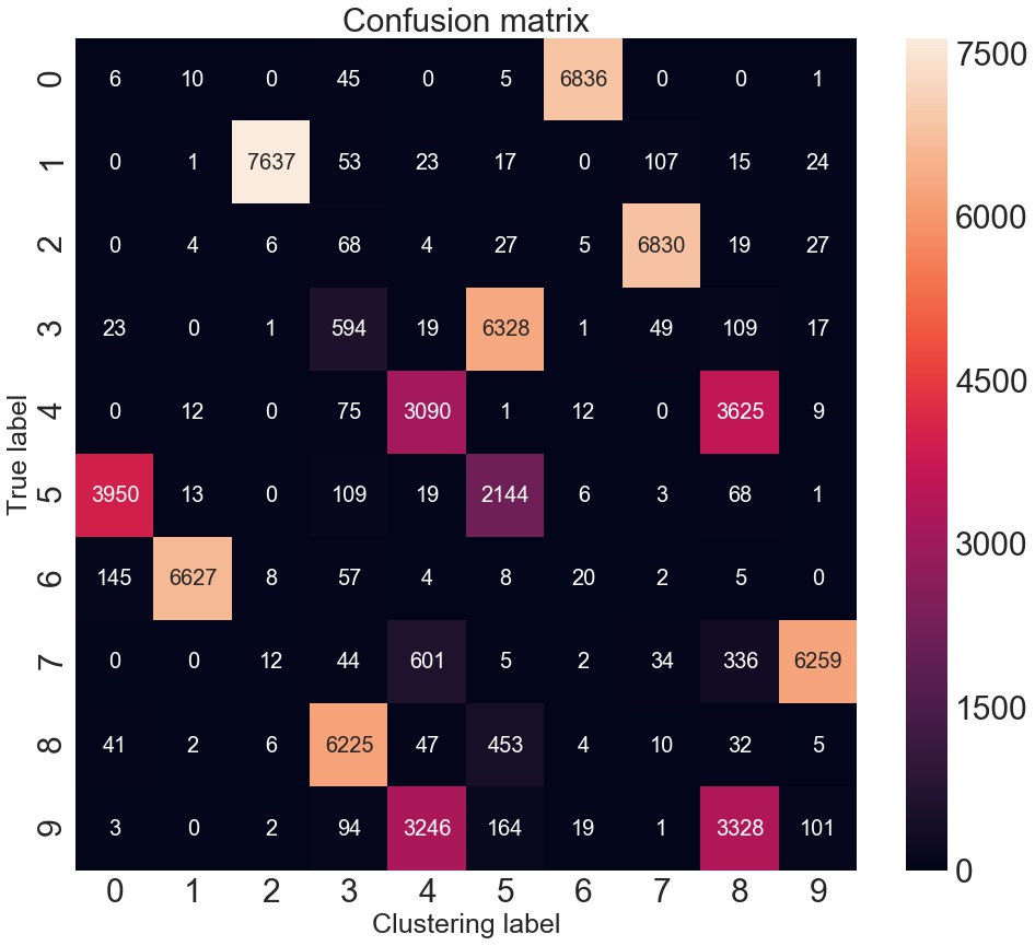
# Acc = 0.79063, nmi = 0.76515, ari = 0.68468 ; loss= 09.7.2. 混淆矩阵
import seaborn as sns
import sklearn.metrics
import matplotlib.pyplot as plt
sns.set(font_scale=3)
confusion_matrix = sklearn.metrics.confusion_matrix(y, y_pred)

plt.figure(figsize=(16, 14))
sns.heatmap(confusion_matrix, annot=True, fmt="d", annot_kws={"size": 20});
plt.title("Confusion matrix", fontsize=30)
plt.ylabel('True label', fontsize=25)
plt.xlabel('Clustering label', fontsize=25)
plt.show()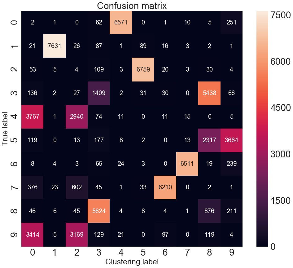
9.8. 多输出同时训练聚类模型和卷积自编码器模型
9.8.1. 网络定义
autoencoder, encoder = autoencoderConv2D_1()
autoencoder.load_weights(save_dir+'/conv_ae_weights.h5')
clustering_layer = ClusteringLayer(n_clusters, name='clustering')(encoder.output)
model = Model(inputs=encoder.input,
              outputs=[clustering_layer, autoencoder.output])

from keras.utils import plot_model
plot_model(model, to_file='model.png', show_shapes=True)
9.8.2. 模型训练
# 采用 K-Means 初始化聚类中心
kmeans = KMeans(n_clusters=n_clusters, n_init=20)
y_pred = kmeans.fit_predict(encoder.predict(x))
model.get_layer(name='clustering').set_weights([kmeans.cluster_centers_])
y_pred_last = np.copy(y_pred)

model.compile(loss=['kld', 'mse'], loss_weights=[0.1, 1], optimizer='adam')

for ite in range(int(maxiter)):
    if ite % update_interval == 0:
        q, _  = model.predict(x, verbose=0)
        # update the auxiliary target distribution p
        p = target_distribution(q)

        # evaluate the clustering performance
        y_pred = q.argmax(1)
        if y is not None:
            acc_ = np.round(acc(y, y_pred), 5)
            nmi_ = np.round(nmi(y, y_pred), 5)
            ari_ = np.round(ari(y, y_pred), 5)
            loss = np.round(loss, 5)
            print('Iter %d: acc = %.5f, nmi = %.5f, ari = %.5f' % (ite, acc_, nmi_, ari_), ' ; loss=', loss)

        # check stop criterion
        delta_label = np.sum(y_pred != y_pred_last).astype(np.float32) / y_pred.shape[0]
        y_pred_last = np.copy(y_pred)
        if ite > 0 and delta_label < tol:
            print('delta_label ', delta_label, '< tol ', tol)
            print('Reached tolerance threshold. Stopping training.')
            break
    idx = index_array[index * batch_size: min((index+1) * batch_size, x.shape[0])]
    loss = model.train_on_batch(x=x[idx], y=[p[idx], x[idx]])
    index = index + 1 if (index + 1) * batch_size <= x.shape[0] else 0

model.save_weights(save_dir + '/conv_b_DEC_model_final.h5')
# model.load_weights(save_dir + '/conv_b_DEC_model_final.h5')

# Final Evaluation
q, _ = model.predict(x, verbose=0)
p = target_distribution(q)  # update the auxiliary target distribution p

# evaluate the clustering performance
y_pred = q.argmax(1)
if y is not None:
    acc_ = np.round(acc(y, y_pred), 5)
    nmi_ = np.round(nmi(y, y_pred), 5)
    ari_ = np.round(ari(y, y_pred), 5)
    loss = np.round(loss, 5)
    print('Acc = %.5f, nmi = %.5f, ari = %.5f' % (acc_, nmi_, ari_), ' ; loss=', loss)
# Acc = 0.82233, nmi = 0.80238, ari = 0.73511  ; loss= 0
9.8.3. 混淆矩阵
9.9. 多输出同时训练聚类模型和全连接自编码器模型
9.9.1. 网络定义
# 数据加载
(x_train, y_train), (x_test, y_test) = mnist.load_data()

x = np.concatenate((x_train, x_test))
y = np.concatenate((y_train, y_test))
x = x.reshape((x.shape[0], -1))
x = np.divide(x, 255.)
n_clusters = len(np.unique(y))
x.shape

dims = [x.shape[-1], 500, 500, 2000, 10]
init = VarianceScaling(scale=1. / 3., mode='fan_in',
                           distribution='uniform')
pretrain_optimizer = SGD(lr=1, momentum=0.9)
pretrain_epochs = 300
batch_size = 256
save_dir = './results'

# 全连接自编码器模型定义
def autoencoder(dims, act='relu', init='glorot_uniform'):
    """
    Fully connected auto-encoder model, symmetric.
    Arguments:
        dims: list of number of units in each layer of encoder.
            dims[0] is input dim,
            dims[-1] is units in hidden layer.
            The decoder is symmetric with encoder.
            So number of layers of the auto-encoder is 2*len(dims)-1
        act: activation,
            not applied to Input, Hidden and Output layers
    return:
        (ae_model, encoder_model),
        Model of autoencoder and model of encoder
    """
    n_stacks = len(dims) - 1
    # input
    input_img = Input(shape=(dims[0],), name='input')
    x = input_img
    # internal layers in encoder
    for i in range(n_stacks-1):
        x = Dense(dims[i + 1],
                  activation=act,
                  kernel_initializer=init,
                  name='encoder_%d' % i)(x)

    # hidden layer, features are extracted from here
    encoded = Dense(dims[-1],
                    kernel_initializer=init,
                    name='encoder_%d' % (n_stacks - 1))(x)

    x = encoded
    # internal layers in decoder
    for i in range(n_stacks-1, 0, -1):
        x = Dense(dims[i],
                  activation=act,
                  kernel_initializer=init,
                  name='decoder_%d' % i)(x)
    # output
    x = Dense(dims[0],
              kernel_initializer=init,
              name='decoder_0')(x)
    decoded = x
    return Model(inputs=input_img,
                 outputs=decoded,
                 name='AE'),
           Model(inputs=input_img,
                 outputs=encoded,
                 name='encoder')

autoencoder, encoder = autoencoder(dims, init=init)
autoencoder.load_weights(save_dir+'/ae_weights.h5')
clustering_layer = ClusteringLayer(n_clusters, name='clustering')(encoder.output)
model = Model(
    inputs=encoder.input,
    outputs=[clustering_layer, autoencoder.output])

from keras.utils import plot_model
plot_model(model, to_file='model.png', show_shapes=True)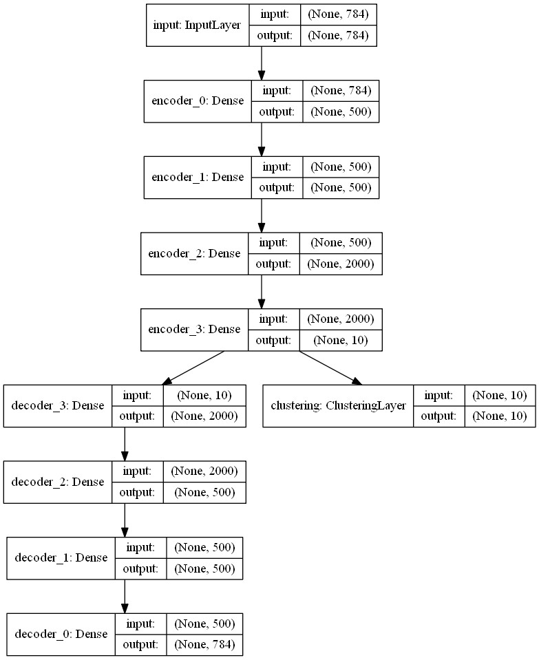
9.9.2. 模型训练
# 采用 K-Means 初始化聚类中心
kmeans = KMeans(n_clusters=n_clusters, n_init=20)
y_pred = kmeans.fit_predict(encoder.predict(x))
model.get_layer(name='clustering').set_weights([kmeans.cluster_centers_])
y_pred_last = np.copy(y_pred)

model.compile(loss=['kld', 'mse'],
              loss_weights=[0.1, 1],
              optimizer=pretrain_optimizer)
# 模型训练
for ite in range(int(maxiter)):
    if ite % update_interval == 0:
        q, _  = model.predict(x, verbose=0)
        # update the auxiliary target distribution p
        p = target_distribution(q)

        # evaluate the clustering performance
        y_pred = q.argmax(1)
        if y is not None:
            acc_ = np.round(acc(y, y_pred), 5)
            nmi_ = np.round(nmi(y, y_pred), 5)
            ari_ = np.round(ari(y, y_pred), 5)
            loss = np.round(loss, 5)
            print('Iter %d: acc = %.5f, nmi = %.5f, ari = %.5f' % (ite, acc_, nmi_, ari_), ' ; loss=', loss)

        # check stop criterion
        delta_label = np.sum(y_pred != y_pred_last).astype(np.float32) / y_pred.shape[0]
        y_pred_last = np.copy(y_pred)
        if ite > 0 and delta_label < tol:
            print('delta_label ', delta_label, '< tol ', tol)
            print('Reached tolerance threshold. Stopping training.')
            break
    idx = index_array[index * batch_size: min((index+1) * batch_size, x.shape[0])]
    loss = model.train_on_batch(x=x[idx], y=[p[idx], x[idx]])
    index = index + 1 if (index + 1) * batch_size <= x.shape[0] else 0

model.save_weights(save_dir + '/b_DEC_model_final.h5')
# model.load_weights(save_dir + '/b_DEC_model_final.h5')

# Final Evaluation
q, _ = model.predict(x, verbose=0)
# update the auxiliary target distribution p
p = target_distribution(q)

# evaluate the clustering performance
y_pred = q.argmax(1)
if y is not None:
    acc_ = np.round(acc(y, y_pred), 5)
    nmi_ = np.round(nmi(y, y_pred), 5)
    ari_ = np.round(ari(y, y_pred), 5)
    loss = np.round(loss, 5)
    print('Acc = %.5f, nmi = %.5f, ari = %.5f' % (acc_, nmi_, ari_), ' ; loss=', loss)
# Acc = 0.95587, nmi = 0.89625, ari = 0.90499  ; loss= 0
9.9.3. 混淆矩阵

19 条评论
请问有pytorch版本的代码吗
没有,keras 的实现.
从混淆矩阵中分析,聚类标签与真实标签为什么不一致?比如聚类标签1与真实标签1匹配,但是为什么说聚类标签1与真实标签7相匹配,没有搞懂?
混淆矩阵反映出来的,聚类标签1和真实标签1相匹配了,6976
请教一下,中间的维度可以不是10维吗?
可以调整
您好,请问处理雷达数据可以用您这种方法吗
不确定哎,不清楚您的雷达数据大概是什么情况.
就是表格形式的数据集,每一条数据记录着一个雷达信号的信息,比如脉冲频率之类的
可能是可以的,1D 卷积?
对的,是1维数据
类似于 1维数据做卷积的套路吧,比如卷积核换成 1xn 或 nx1,比如这个 https://zhuanlan.zhihu.com/p/259575697
好的,谢谢作者大大啦,感谢你
请问电能质量扰动的各采样点数据集,可以用卷积自编码器吗,为啥总是提示维度错误。
电能质量扰动的各采样点数据集? 这个没试过,理论上是可以的.
博主,你好,请问卷积自动编码器有没有完整的源码。 谢谢您
请教博主,卷积自编码器做的效果比全连接还差吗?
没具体操作下采用卷积自编码器处理同样的问题,所以没有进行对比,对于图像的话,理论上应该不会差吧
谢谢,受教啦