关于 Pytorch 的 nn.torch.Conv2d 的记录与理解.
CLASS torch.nn.Conv2d(in_channels, out_channels, kernel_size, stride=1, padding=0, dilation=1, groups=1, bias=True)假设 Conv2d 的输入 input 尺寸为 $(N, C_{in}, H_{in}, W_{in})$,输出 output 尺寸为 $(N, C_{out}, H_{out}, W_{out})$,有:
$out(N_i, C_{out_j}) = bias(C_{out_j}) + \sum _{k=0}^{C_{in} - 1} weight(C_{out_j}, k) * input(N_i, k)$
其中,$*$ 是 2D cross-correlation 操作. $N$ - batch size, $C$ - channels 数, $H$ - Hight, $W$ - Width.
- [1] - kernel_size
- [2] - stride - 步长
- [3] - padding - 每一维补零的数量
- [4] - dilation - 控制 kernel 点之间的空间距离(the spacing between the kernel points). 带孔卷积(atrous conv). 参考 dilated-convolution-animations.
- [5] - groups - 控制 inputs 和 outputs 间的关联性(分组). 其中,要求
in_channels和out_channels必须都可以被groups整除.
$H_{out} = \frac{H_{in} + 2\times padding[0] - dilation[0] \times (kernel\_size[0] - 1) - 1}{stride[0]} + 1$
$W_{out} = \frac{W_{in} + 2\times padding[1] - dilation[1] \times (kernel\_size[1] - 1) - 1}{stride[1]} + 1$
1. Demo
import torch
import torch.nn as nn

# With square kernels and equal stride
m = nn.Conv2d(16, 33, 3, stride=2)
 # non-square kernels and unequal stride and with padding
m = nn.Conv2d(16, 33, (3, 5), stride=(2, 1), padding=(4, 2))
# non-square kernels and unequal stride and with padding and dilation
m = nn.Conv2d(16, 33, (3, 5), stride=(2, 1), padding=(4, 2), dilation=(3, 1))
input = torch.randn(20, 16, 50, 100)
output = m(input)
2. 关于 groups 参数
对于 groups 参数,用于分解 inputs 和 outputs 间的关系,分组进行卷积操作.
[1] - groups=1,所有输入进行卷积操作,得到输出.
[2] - groups=2,等价于有两个并列 conv 操作,每个的输入是一半的 input_channels,并输出一半 - 的 output_channels,然后再进行链接.
[3] - groups=in_channels,每个 input channel 被其自己的 filters 进行卷积操作,尺寸为 $\frac{C_{out}}{C_{in}}$.
当 group=in_channels 且 out_channels = K * in_channels,其中,K 是正整数,此时的操作被称为 depthwise convolution.
换句话说,对于输出尺寸为 $(N, C_{in}, H_{in}, W_{in})$, depthwise multiplier 为 K 的depthwise convolution 可以构建为:
$(in\_channels = C_{in}, out\_channels=C_{in} \times K,..., groups=C_{in})$
2.1 groups 参数示例 demo
import numpy as np
import cv2
import matplotlib.pyplot as plt

import torch
import torch.nn as nn
import torchvision.transforms.functional as F

img = cv2.imread('test.jpg')
img_224 = cv2.resize(img, (224, 224), cv2.INTER_LINEAR)
img_224 = cv2.cvtColor(img_224, cv2.COLOR_BGR2RGB)

img_tensor = torch.from_numpy(np.moveaxis(img_224 / (255. if img_224.dtype == np.uint8 else 1), -1, 0).astype(np.float32))
inputs = torch.unsqueeze(img_tensor, 0)

conv = nn.Conv2d(in_channels=3, out_channels=6, kernel_size=7, stride=2, padding=3, groups=3, bias=False)
nn.init.xavier_uniform_(conv.weight.data, gain=nn.init.calculate_gain('relu'))
print(conv.weight.data.size())
print(conv.weight.data)

output=conv(inputs)
print(output)groups决定了将原输入in_channels 分为几组,而每组channel重用几次,由out_channels/groups计算得到,这也说明了为什么需要groups能供被out_channels与in_channels整除. - pyotrch_nn.Conv2d中groups参数的理解
3. 卷积层原理及例示[转]
卷积层是用一个固定大小的矩形区去席卷原始数据,将原始数据分成一个个和卷积核大小相同的小块,然后将这些小块和卷积核相乘输出一个卷积值(注意这里是一个单独的值,不再是矩阵了).
卷积的本质就是用卷积核的参数来提取原始数据的特征,通过矩阵点乘的运算,提取出和卷积核特征一致的值,如果卷积层有多个卷积核,则神经网络会自动学习卷积核的参数值,使得每个卷积核代表一个特征.
3.1 以 conv1d 举例说明卷积过程的计算
conv1d是一维卷积,它和conv2d的区别在于只对宽度进行卷积,对高度不卷积.
函数定义:
torch.nn.functional.conv1d(input, weight, bias=None, stride=1, padding=0, dilation=1, groups=1)参数说明:
- input:输入的Tensor数据,格式为(batch, channels, W),三维数组,第一维度是样本数量,第二维度是通道数或者记录数,三维度是宽度.
- weight:卷积核权重,也就是卷积核本身. 是一个三维数组,(out_channels, in_channels/groups, kW). out_channels 是卷积核输出层的神经元个数,也就是这层有多少个卷积核;in_channels是输入通道数;kW是卷积核的宽度.
- bias:位移参数,可选项,一般也不用管.
- stride:滑动窗口,默认为1,指每次卷积对原数据滑动1个单元格.
- padding:是否对输入数据填充0. Padding可以将输入数据的区域改造成是卷积核大小的整数倍,这样对不满足卷积核大小的部分数据就不会忽略了. 通过padding参数指定填充区域的高度和宽度,默认0(填充区域为0,不填充).
- dilation:卷积核之间的空格,默认1.
- groups:将输入数据分组,通常不用管这个参数.
import torch
import torch.nn as nn
import torch.nn.functional as F
from torch.autograd import Variable


print("conv1d sample")

a=range(16)
x = Variable(torch.Tensor(a))
x=x.view(1,1,16)
print("x variable:", x)

b=torch.ones(3)
b[0]=0.1
b[1]=0.2
b[2]=0.3
weights = Variable(b) #torch.randn(1,1,2,2)) #out_channel*in_channel*H*W
weights=weights.view(1,1,3)
print ("weights:",weights)

y=F.conv1d(x, weights, padding=0)
print ("y:",y)
输出结果为:
conv1d sample
x variable: tensor([[[  0.,   1.,   2.,   3.,   4.,   5.,   6.,   7.,   8.,   9.,  10.,  11.,  12.,  13.,  14.,  15.]]])
weights: tensor([[[ 0.1000,  0.2000,  0.3000]]])
y: tensor([[[ 0.8000,  1.4000,  2.0000,  2.6000,  3.2000,  3.8000,  4.4000,  5.0000,  5.6000,  6.2000,  6.8000,  7.4000,  8.0000,  8.6000]]])
它是怎么计算的:
(1) 原始数据大小是0-15的一共16个数字,卷积核宽度是3,向量是[0.1, 0.2, 0.3]. 第一个卷积是对 x[0:3] 共3个值 [0,1,2] 进行卷积,公式如下:
0x0.1+1x0.2+2x0.3=0.8
(2) 对第二个目标卷积,是 x[1:4 ]共3个值 [1,2,3] 进行卷积,公式如下:
1x0.1+2x0.2+3x0.3=1.4
看到和计算结果完全一致.
conv1d 示意图如下:
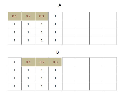
conv1d 和 conv2d 的区别就是只对宽度卷积,不对高度卷积. 最后的结果的宽度是原始数据的宽度减去卷积核的宽度再加上1,这里就是14.
Pytorch卷积层原理和示例