原文:目标检测YOLO、SSD、RetinaNet、Faster RCNN、Mask RCNN(1) - 2019.01.01
作者:油腻小年轻 - 简书
学习,备忘.
本文分析的目标检测网络的源码都是基于Keras, Tensorflow. 最近看了李沐大神的新作《动手学深度学习》,感觉MxNet框架用起来很讨喜,Github上也有YOLOV3,SSD,Faster RCNN,RetinaNet,Mask RCNN这5种网络的MxNet版源码,不过考虑到Tensorflow框架的普及,还是基于Keras来分析目标检测网络的代码实现.
1. 目标检测基础
1.1. 准确率判断
分对的正反例样本数 / 样本总数.
用于评估模型的全局准确程度,因为包含的信息有限,一般不用于评估模型的性能
1.2. 精确率与召回率
| Predicted Negative | Predicted Positive | |
|---|---|---|
| Negative Cases | TN: 9760 | FP: 140 |
| Positive Cases | FN: 40 | TP: 60 |
一些相关的定义.
假设现在有这样一个测试集,测试集中的图片只由大雁和飞机两种图片组成,假设分类系统最终的目的是:能取出测试集中所有飞机的图片,而不是大雁的图片.
- True positives : 正样本被正确识别为正样本,飞机的图片被正确的识别成了飞机.
- True negatives: 负样本被正确识别为负样本,大雁的图片没有被识别出来,系统正确地认为它们是大雁.
- False positives: 假的正样本,即负样本被错误识别为正样本,大雁的图片被错误地识别成了飞机.
- False negatives: 假的负样本,即正样本被错误识别为负样本,飞机的图片没有被识别出来,系统错误地认为它们是大雁.
Precision 其实就是在识别出来的图片中,True positives所占的比率. 也就是本假设中,所有被识别出来的飞机中,真正的飞机所占的比例.
$$ Precision = \frac{TP}{TP + FP} $$
Recall 是测试集中所有正样本样例中,被正确识别为正样本的比例. 也就是本假设中,被正确识别出来的飞机个数与测试集中所有真实飞机的个数的比值.
$$ Recall = \frac{TP}{TP + FN} $$
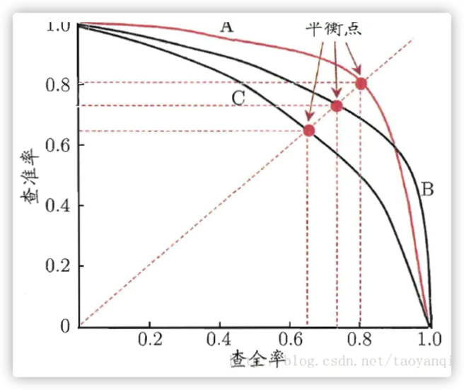
- Precision-recall 曲线:改变识别阈值,使得系统依次能够识别前K张图片,阈值的变化同时会导致Precision与Recall值发生变化,从而得到曲线.
如果一个分类器的性能比较好,那么它应该有如下的表现:在Recall值增长的同时,Precision的值保持在一个很高的水平. 而性能比较差的分类器可能会损失很多 Precision 值才能换来 Recall 值的提高. 通常情况下,文章中都会使用Precision-recall曲线,来显示出分类器在Precision与Recall之间的权衡.
以下面的 p-r 图为例,我们可以看到PR曲线C是包含于A和B,那么我们可以认为A和B的性能是优于C.
1.3. 平均精度AP 与多类别平均精度mAP
AP 就是Precision-recall 曲线下面的面积,通常来说一个越好的分类器,AP值越高.
mAP 是多个类别AP的平均值. 这个mean的意思是对每个类的AP再求平均,得到的就是mAP的值,mAP的大小一定在[0,1]区间,越大越好. 该指标是目标检测算法中最重要的一个.
1.4. IoU
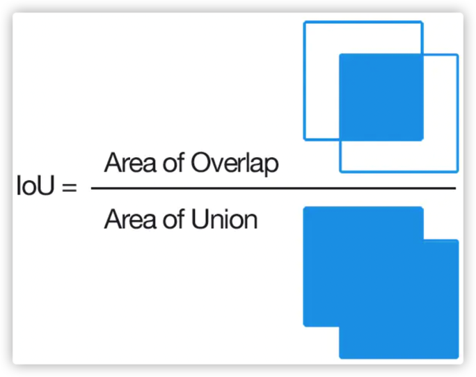
IoU这一值,可以理解为系统预测出来的框与原来图片中标记的框的重合程度.
计算方法即检测结果Detection Result与 Ground Truth 的交集比上它们的并集,即为检测的准确率.
IoU正是表达这种bounding box和groundtruth的差异的指标:
1.5. 非极大值抑制(NMS)
Non-Maximum Suppression 就是需要根据 score 矩阵和 region 的坐标信息,从中找到置信度比较高的bounding box. 对于有重叠在一起的预测框,只保留得分最高的那个.
[1] - NMS计算出每一个bounding box的面积,然后根据score进行排序,把score最大的bounding box作为队列中首个要比较的对象.
[2] - 计算其余bounding box与当前最大score与box的IoU,去除IoU大于设定的阈值的bounding box,保留小的IoU得预测框.
[3] - 然后重复上面的过程,直至候选bounding box为空.
最终,检测了bounding box的过程中有两个阈值,一个就是IoU,另一个是在过程之后,从候选的bounding box中剔除score小于阈值的bounding box.
需要注意的是:Non-Maximum Suppression一次处理一个类别,如果有N个类别,Non-Maximum Suppression就需要执行N次.
1.6. 卷积神经网络
卷积神经网络仿造生物的视知觉(visual perception)机制构建,可以进行监督学习非监督学习,其隐含层内的卷积核参数共享和层间连接的稀疏性使得卷积神经网络能够以较小的计算量对格点化(grid-like topology)特征,例如像素和音频进行学习、有稳定的效果且对数据没有额外的特征工程(feature engineering)要求.
1.7. One Stage & Two Stage
目标检测模型目的是自动定位出图像中的各类物体,不仅可以给出物体的类别判定,也可以给出物体的定位. 目前主流的研究分为两类:One Stage 和 Two stage, 前者是图像经过网络的计算图,直接预测出图中物体的类别和位置;后者则先提取出物体的候选位置(Region Proposal),然后再对物体进行分类,当然这个时候一般也会对筛选出来的目标做一次定位的精修,达到更加准确的目的.
YOLOV3,SSD,RetinaNet都属于one stage类型的网络,这类网络的特点是训练和识别速度快,但是精度欠佳.
Faster RCNN和Mask RCNN属于two stage类型的网络,相比于one stage,识别精度上有所提升,但是训练和识别速度比不上one stage类型的网络.
2. YOLOV3
2.1. YOLOV3 网络结构
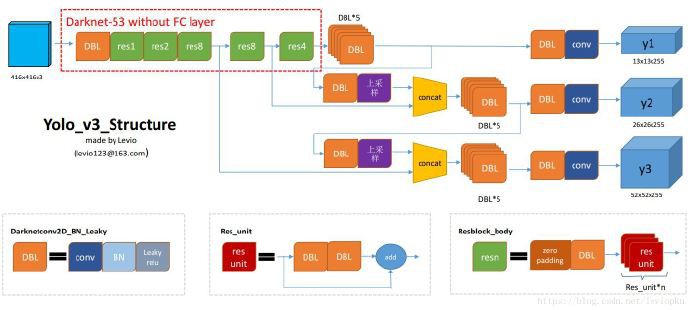
From yolo系列之yolo v3【深度解析】- 木盏 - CSDN
DBL: 卷积层Conv + 批标准化层BN + Leaky Relu.
res(n): n 代表这个 res_block 内含有多少个 res_unit,这点借鉴了ResNet的残差结构,使用这种结构的目的是为了加深网络深度
concat: 将DarkNet中的某一层与之前的某层的上采样.
YOLOV3 流程如下:
[1] - 调整输入图像的大小为416 × 416(32的倍数)
[2] - 图像向前传播的过程中经过一个 1 个DBL层和 5 个res_block,每经过一个res_block,图像的size 都要减半,此时图像的 size为416 / 32(2的5次方) = 13 * 13.
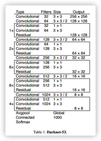
[3] - 下图是一张DarkNet-53的结构图,然而 YOLOV3 经过前面的 res_block 后不是继续采用接下来的 Avgpool 平均池化层,Connected,全连接层,而是继续经过5个DBL层.
[4] - 接下来有两步操作:
(4.1) - 经过一个 DBL层和卷积层 conv 得到输出y1(13 13 255),这里的255是9 / 3 * (4 + 1 + 80). 对这几个数字的说明如下:
- 9 是 anchors的数量,这里的anchor的数量是通过聚类得到的.
- 除以3是因为最终的输出的特征图有3个 scale (13,26,52),13 * 13 对应的是9个anchors里top3 大的锚框.
- 4代表的每个锚框中心的横坐标x,纵坐标y,宽度w,高度h.
- 1和80分别表示背景和80目标种类的概率
(4.2) - 通过一个DBL和一个上采样层和 res_block4 的输出连接起来,然后经过5个DBL层.
[5] - 步骤(4.2)的结果也有两步操作:
(5.1) - 经过一个 DBL 层和卷积层 conv 得到输出y2(26 26 255),26是因为res_block4的输出特征图大小为26,而步骤(4.1)的输入经过上采样的操作后特征图大小也从13变成了26.
(5.2) - 通过一个DBL和一个上采样层和res_block3的输出连接起来,然后经过5个DBL层.
[6] - 将步骤(5.2) 的结果经过一个 DBL 层和一个上采样层与 res_block3 的输出连接起来,再经过6(5+1)个 DBL 层和一个卷积层conv得到y3(52 52 255).
2.2. YOLOV3 Loss
使用YOLO做预测,结果会给出图像中物体的中心点坐标(x,y),目标是否是一个物体的置信度C以及物体的类别,比如说person,car,ball等等.
图像经过之前的计算图前向传播得到 3 个 scale 的输出y1(13),y2(26),y3(52),用yolo_outputs代表这3个变量.
将原始图片(416 * 416)分别除以32,16,8得到与y1,y2,y3大小匹配的ground_truth,在源码中用y_true表示.
计算损失的时候需要把预测出来的结果与ground truth box之间的差距表现出来,下面是YOLOV1的loss function:
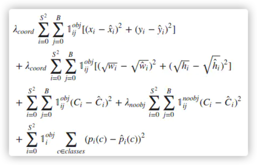
2.2.1. 坐标误差
λcoord 在 YOLOV1 中默认为 5,因为目标的定位是最重要的部分,所以给定位损失一个比较高的权重. 但是在看代码的时候发现这个值变成了 $2 - w \cdot h$ (w, h 都归一化到[0,1]),应该是降低了一些权重,同时将物体的大小考虑进去,从公式中可以发现小的物体拥有更高的权重,因为对于小物体,几个像素的误差带来的影响是高于大的物体.
对于中心点坐标的(x,y)的计算也从 MSE 均方差误差变成了 binary_crossentropy 二分类交叉熵,为啥变成这个可能有点玄学在里面,反正对于坐标的损失计算,作者认为MSE是没问题的.
计算宽高的误差之前先看下下面这张图:
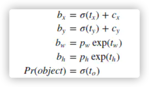
网络预测出来的中心点坐标和宽高分别为 $t_x, t_y, t_w, t_h$,通过计算得到边框的中心坐标 $b_x, b_y$,和边框的宽$b_w$,高$b_h$.
$c_x, c_y$ 是位移偏差offset,$\sigma ()$ 函数为logistic函数,将坐标归一化到[0,1].
最终得到的 $b_x, b_y$ 为归一化后的相对于 grid cell 的值. $p_w,p_h$ 为anchor的宽和高.
实际在使用中,作者为了将 $b_w, b_h$ 也归一化到[0,1],实际程序中的 $p_w, p_h$ 为 anchor 的宽,高和featuremap 的宽,高的比值. 最终得到的$p_w, p_h$ 为归一化后相对于 anchor 的值.
raw_true_wh = K.log(y_true[l][..., 2:4] / anchors[anchor_mask[l]] * input_shape[::-1])
raw_true_wh = K.switch(object_mask, raw_true_wh, K.zeros_like(raw_true_wh)) # avoid log(0)=-inf
#......此处省略中间的一些代码,直接看w和h的误差计算
wh_loss = object_mask * box_loss_scale * 0.5 * K.square(raw_true_wh-raw_pred[...,2:4])
YOLOV3 跟 YOLOV1 对于宽高的损失计算也有些区别,YOLOV1是 $(\sqrt {w} - \sqrt{w'} )^2$;YOLOV3是$(log(w) - log(w')))^2$,不过效果是一样的,都是提高对于小目标的预测敏感度. 举个简单的例子,同样是10个像素的误差,一个大的目标真实的宽为100,预测出来为110;而一个小的目标真实宽度为10,预测出来是20,让我们来通过这个公式计算一下误差:
0.5 * (log(110) - log(100))^2 = 0.00085667719
0.5 * (log(20) - log(10))^2 = 0.04530952914
可以看出对于小的物体,对于同样像素大小的误差,惩罚比较大
2.2.2. IOU 误差
对于有边界框的物体,计算出置信度和1之间的差值;
对于背景,我们需要计算出置信度与0之间的差值,当然距离计算公式还是用二分类交叉熵.
λnoobj在源码中没有找到这个参数,YOLOV1是设置来减少正反例分布不均匀带来的误差的,作者为什么要这么做,作者暂还没找到原因,猜测是对于这种分布不均衡问题我们没有必要去干预它,顺其自然就好.
2.2.3. 分类误差
这个就比较直观了.
class_loss = object_mask * K.binary_crossentropy(
    true_class_probs,
    raw_pred[...,5:],
    from_logits=True)
2.3. YOLOV3 检测示例
借助Opencv,keras-yolov3可以实现影像的目标检测:
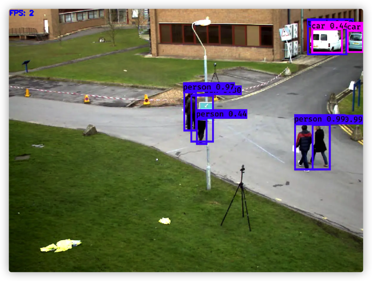
当然也可以进行图片的目标检测:
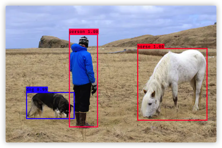
2.4. YOLOV3 检测流程代码
检测代码可以见 yolo_video.py,其中 function detect_video 是调用了Opencv对影像处理的接口,然后复用了接口detect_image. 对于目标检测的流程可以总结为以下几个步骤:
1. 初始化
self.__dict__.update(self._defaults) # set up default values
        self.__dict__.update(kwargs) # and update with user overrides
        self.class_names = self._get_class()
        self.anchors = self._get_anchors()
        self.sess = K.get_session()
        self.boxes, self.scores, self.classes = self.generate()
载入分类的类名('car','house','people'......)
载入聚类算法计算得到的9个锚框.
初始化tensorflow计算图session
载入训练好的Model.
    def generate(self):
        model_path = os.path.expanduser(self.model_path)
        assert model_path.endswith('.h5'), 'Keras model or weights must be a .h5 file.'

        # Load model, or construct model and load weights.
        num_anchors = len(self.anchors)
        num_classes = len(self.class_names)
        is_tiny_version = num_anchors==6 # default setting
        try:
            self.yolo_model = load_model(model_path, compile=False)
        except:
            self.yolo_model = tiny_yolo_body(
                Input(shape=(None,None,3)),
                num_anchors//2,
                num_classes)
                if is_tiny_version else
                    yolo_body(Input(shape=(None,None,3)),
                              num_anchors//3,
                              num_classes)
            # make sure model, anchors and classes match
            self.yolo_model.load_weights(self.model_path)
        else:
            assert self.yolo_model.layers[-1].output_shape[-1] == \
                num_anchors/len(self.yolo_model.output) * (num_classes + 5), \
                'Mismatch between model and given anchor and class sizes'

        print('{} model, anchors, and classes loaded.'.format(model_path))
定义网络输出的计算,输出的shape为[(?,13,13,255),(?,26,26,255),(?,52,52,255)],?表示batch_size,如果一次检测一张图片的话,这个数字为1. 原则上只要GPU的内存够,可以扩大 batch_size.
self.input_image_shape = K.placeholder(shape=(2, ))
if self.gpu_num>=2:
    self.yolo_model = multi_gpu_model(self.yolo_model, gpus=self.gpu_num)
    boxes, scores, classes = yolo_eval(self.yolo_model.output,
                                       self.anchors,
                                       len(self.class_names),
                                       self.input_image_shape,
                                       score_threshold=self.score,
                                       iou_threshold=self.iou)
    return boxes, scores, classes
接下来要得到正确的 box 坐标还有 box_score (这个坐标是否包含物体的概率 * 分类的得分)
def yolo_correct_boxes(box_xy, box_wh, input_shape, image_shape):
    '''
    Get corrected boxes
    '''
    box_yx = box_xy[..., ::-1]
    box_hw = box_wh[..., ::-1]
    input_shape = K.cast(input_shape, K.dtype(box_yx))
    image_shape = K.cast(image_shape, K.dtype(box_yx))
    new_shape = K.round(image_shape * K.min(input_shape/image_shape))
    offset = (input_shape-new_shape)/2./input_shape
    scale = input_shape/new_shape
    box_yx = (box_yx - offset) * scale
    box_hw *= scale

    box_mins = box_yx - (box_hw / 2.)
    box_maxes = box_yx + (box_hw / 2.)
    boxes =  K.concatenate([
        box_mins[..., 0:1],  # y_min
        box_mins[..., 1:2],  # x_min
        box_maxes[..., 0:1],  # y_max
        box_maxes[..., 1:2]  # x_max
    ])

    # Scale boxes back to original image shape.
    boxes *= K.concatenate([image_shape, image_shape])
    return boxes

def yolo_boxes_and_scores(feats, anchors, num_classes, input_shape, image_shape):
    '''
    Process Conv layer output
    '''
    box_xy, box_wh, box_confidence, box_class_probs = yolo_head(
        feats,anchors, num_classes, input_shape)
    boxes = yolo_correct_boxes(box_xy, box_wh, input_shape, image_shape)
    boxes = K.reshape(boxes, [-1, 4])
    box_scores = box_confidence * box_class_probs
    box_scores = K.reshape(box_scores, [-1, num_classes])
    return boxes, box_scores

def yolo_eval(yolo_outputs,
              anchors,
              num_classes,
              image_shape,
              max_boxes=20,
              score_threshold=.6,
              iou_threshold=.5):
    """
    Evaluate YOLO model on given input and return filtered boxes.
    """
    num_layers = len(yolo_outputs)
    anchor_mask = [[6,7,8], [3,4,5], [0,1,2]] if num_layers==3 else [[3,4,5], [1,2,3]] # default setting
    input_shape = K.shape(yolo_outputs[0])[1:3] * 32
    boxes = []
    box_scores = []
    for l in range(num_layers):
        _boxes, _box_scores = yolo_boxes_and_scores(
            yolo_outputs[l],
            anchors[anchor_mask[l]],
            num_classes,
            input_shape,
            image_shape)
        boxes.append(_boxes)
        box_scores.append(_box_scores)
    boxes = K.concatenate(boxes, axis=0)
    box_scores = K.concatenate(box_scores, axis=0)
这个时候,过滤掉那些得分低于score_threshold(0.6)的候选框:
mask = box_scores >= score_threshold
max_boxes_tensor = K.constant(max_boxes, dtype='int32')
再调用NMS算法,将那些同一分类重合度过高的候选框给筛选掉:
boxes_ = []
scores_ = []
classes_ = []
for c in range(num_classes):
    # TODO: use keras backend instead of tf.
    class_boxes = tf.boolean_mask(boxes, mask[:, c])
    class_box_scores = tf.boolean_mask(box_scores[:, c], mask[:, c])
    nms_index = tf.image.non_max_suppression(
        class_boxes,
        class_box_scores,
        max_boxes_tensor,
        iou_threshold=iou_threshold)
    class_boxes = K.gather(class_boxes, nms_index)
    class_box_scores = K.gather(class_box_scores, nms_index)
    classes = K.ones_like(class_box_scores, 'int32') * c
    boxes_.append(class_boxes)
    scores_.append(class_box_scores)
    classes_.append(classes)
boxes_ = K.concatenate(boxes_, axis=0)
scores_ = K.concatenate(scores_, axis=0)
classes_ = K.concatenate(classes_, axis=0)

return boxes_, scores_, classes_
现在我们得到了目标框以及对应的得分和分类:
self.boxes, self.scores, self.classes = self.generate()2.5. YOLOV3 图片预处理代码
保持图片的比例,其余部分用灰色填充:
def letterbox_image(image, size):
    '''
    resize image with unchanged aspect ratio using padding.
    '''
    iw, ih = image.size
    w, h = size
    scale = min(w/iw, h/ih)
    nw = int(iw*scale)
    nh = int(ih*scale)

    image = image.resize((nw,nh), Image.BICUBIC)
    new_image = Image.new('RGB', size, (128,128,128))
    new_image.paste(image, ((w-nw)//2, (h-nh)//2))

    return new_image
if self.model_image_size != (None, None):
assert self.model_image_size[0]%32 == 0, 'Multiples of 32 required'
assert self.model_image_size[1]%32 == 0, 'Multiples of 32 required'
boxed_image = letterbox_image(
image, tuple(reversed(self.model_image_size)))
else:
new_image_size = (image.width - (image.width % 32),
image.height - (image.height % 32))
boxed_image = letterbox_image(image, new_image_size) #
image_data = np.array(boxed_image, dtype='float32')像素各通道值归一化:
image_data /= 255.
image_data = np.expand_dims(image_data, 0)  # Add batch dimension.
2.6. YOLOV3 前向计算代码
out_boxes, out_scores, out_classes = self.sess.run(
    [self.boxes, self.scores, self.classes],
    feed_dict={self.yolo_model.input: image_data,
               self.input_image_shape: [image.size[1], image.size[0]],
               K.learning_phase(): 0}
)

print('Found {} boxes for {}'.format(len(out_boxes), 'img'))
最后就是调用PIL的一些辅助接口将这些目标框和得分绘制在原始图片上.
3. 目标检测识别精度与速度
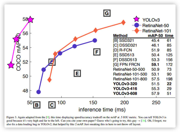
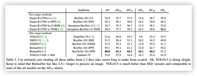
上面两张图已经很能说明YOLOV3的性能,不仅可以保障较高的精度,在速度上更是遥遥领先. .
1 条评论
Keras 在那呢?