节选 From:Multi-label Classification With Keras
基于 Keras 的服装多标签分类
1. 问题描述
Clothing type: Shirts, Dresses, Pants, Shoes, etc.
Color: Red, Blue, Green, Black, etc.
Texture/appearance: Cotton(棉), Wool(羊毛), silk(丝), Tweed(麻), etc.
这里主要对 Clothing type 服装类型 和 Color 服装颜色 两种 labels 进行分类.
如:
2. 基于 Keras 的 Multi-label 分类
主要包括四部分:
- Multi-label 分类数据集
- Keras 网络结构 - SmallerVGGNet 简介
- SmallerVGGNet 网络的实现和训练
- 分类器测试
2.1 Multi-label 分类数据集

Figure 1. Mutli-label 分类服装数据集.
数据集共有 2167 张图片, 六个类别, 具体如:
- Black jeans (344 images)
- Blue dress (386 images)
- Blue jeans (356 images)
- Blue shirt (369 images)
- Red dress (380 images)
- Red shirt (332 images)
目标场景:采用 CNNs 同时预测服装类型和服装颜色.
Multi-label 分类数据集的构建,可参考: How to (quickly) build a deep learning image dataset
2.2 Multi-label 分类项目组织结构
├── classify.py
├── dataset
│   ├── black_jeans [344 entries
│   ├── blue_dress [386 entries]
│   ├── blue_jeans [356 entries]
│   ├── blue_shirt [369 entries]
│   ├── red_dress [380 entries]
│   └── red_shirt [332 entries]
├── examples
│   ├── example_01.jpg
│   ├── example_02.jpg
│   ├── example_03.jpg
│   ├── example_04.jpg
│   ├── example_05.jpg
│   ├── example_06.jpg
│   └── example_07.jpg
├── fashion.model
├── mlb.pickle
├── plot.png
├── pyimagesearch
│   ├── __init__.py
│   └── smallervggnet.py
├── search_bing_api.py
└── train.py
主要有 6 个文件和 3 个目录:
- search_bing_api.py - 用于快速创建图片数据集(这里不必运行).
- train.py - 分类器模型训练脚本.
- fashion.model - 训练的模型保存的 Keras 文件. 用于分类器测试.
- mlb.pickle - 由
train.py模型训练时创建的 scikit-learnMultiLabelBinarizerpickle 文件 - 以顺序数据结构存储了各类别的名字. - plot.png - 模型训练时生成的图像文件,用于 accuracy/loss 和过拟合情况的可视化.
- classifier.py - 分类器模型测试脚本.
- dataset - 数据集路径,其内的每个子目录分别表示一个类别的图像. 便于数据集的组织化;便于从给定图像路径提取类别标签名.
- pyimagesearch - CNNs网路路径,包含了 Keras 网络结构模块.
- examples - 测试样例图片,7 张.
# scikit-learn 的 MultiLabelBinarizer 函数例示
>>> from sklearn.preprocessing import MultiLabelBinarizer
>>> labels = [
...     ("blue", "jeans"),
...     ("blue", "dress"),
...     ("red", "dress"),
...     ("red", "shirt"),
...     ("blue", "shirt"),
...     ("black", "jeans")
... ]
>>> mlb = MultiLabelBinarizer()
>>> mlb.fit(labels)
MultiLabelBinarizer(classes=None, sparse_output=False)
>>> mlb.classes_
array(['black', 'blue', 'dress', 'jeans', 'red', 'shirt'], dtype=object)
>>> mlb.transform([("red", "dress")])
array([[0, 0, 1, 0, 1, 0]])
2.3 Multi-label 分类的 Keras 网络结构
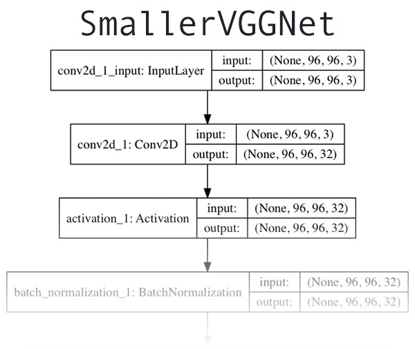
Figure 2. SmallVGGNet 结构
VGGNet - Very Deep Convolutional Networks for Large Scale Image Recognition
VGGNet-like 的网络结构主要特点:
- 只使用 3x3 conv 层
- 采用 max-pooling 层减少尺寸
- 网络输出端为全连接层 + softmax 分类器
# smallervggnet.py
from keras.models import Sequential
from keras.layers.normalization import BatchNormalization
from keras.layers.convolutional import Conv2D
from keras.layers.convolutional import MaxPooling2D
from keras.layers.core import Activation
from keras.layers.core import Flatten
from keras.layers.core import Dropout
from keras.layers.core import Dense
from keras import backend as K


class SmallerVGGNet:
    @staticmethod
    def build(width, height, depth, classes, finalAct="softmax"):
        # classes: 类别标签数(而非类别标签.)
        # finalAct: 默认为 softmax, multi-label 分类中采用 sigmoid.

        # initialize the model along with the input shape to be
        # "channels last" and the channels dimension itself
        model = Sequential()
        inputShape = (height, width, depth)
        chanDim = -1

        # if we are using "channels first", update the input shape
        # and channels dimension
        if K.image_data_format() == "channels_first":
            inputShape = (depth, height, width)
            chanDim = 1

        # 网络层 CONV => RELU => POOL
        model.add(Conv2D(32, (3, 3), padding="same",
                         input_shape=inputShape)) # 32 个 3x3
        model.add(Activation("relu"))
        model.add(BatchNormalization(axis=chanDim))
        model.add(MaxPooling2D(pool_size=(3, 3)))
        model.add(Dropout(0.25)) # 25% 的 dropout
        # Dropout 层随机丢弃当前层传递到下一网络层的部分节点.

        # 网络层 (CONV => RELU) * 2 => POOL
        model.add(Conv2D(64, (3, 3), padding="same"))
        model.add(Activation("relu"))
        model.add(BatchNormalization(axis=chanDim))
        model.add(Conv2D(64, (3, 3), padding="same"))
        model.add(Activation("relu"))
        model.add(BatchNormalization(axis=chanDim))
        model.add(MaxPooling2D(pool_size=(2, 2)))
        model.add(Dropout(0.25))

        # 网络层 (CONV => RELU) * 2 => POOL
        model.add(Conv2D(128, (3, 3), padding="same"))
        model.add(Activation("relu"))
        model.add(BatchNormalization(axis=chanDim))
        model.add(Conv2D(128, (3, 3), padding="same"))
        model.add(Activation("relu"))
        model.add(BatchNormalization(axis=chanDim))
        model.add(MaxPooling2D(pool_size=(2, 2)))
        model.add(Dropout(0.25))

        # 网络层 first (and only) set of FC => RELU layers
        model.add(Flatten())
        model.add(Dense(1024))
        model.add(Activation("relu"))
        model.add(BatchNormalization())
        model.add(Dropout(0.5))

        # softmax classifier
        model.add(Dense(classes))
        model.add(Activation(finalAct))

        return model
2.4 Multi-label 分类的 Keras 模型实现
模型训练脚本 train.py.
import matplotlib
matplotlib.use("Agg")
from keras.preprocessing.image import ImageDataGenerator
from keras.optimizers import Adam
from keras.preprocessing.image import img_to_array
from sklearn.preprocessing import MultiLabelBinarizer
from sklearn.model_selection import train_test_split
from pyimagesearch.smallervggnet import SmallerVGGNet
import matplotlib.pyplot as plt
from imutils import paths
import numpy as np
import argparse
import random
import pickle
import cv2
import os
# 参数配置
ap = argparse.ArgumentParser()
ap.add_argument("-d", "--dataset", required=True,
help="path to input dataset (i.e., directory of images)")
ap.add_argument("-m", "--model", required=True,
help="path to output model")
ap.add_argument("-l", "--labelbin", required=True,
help="path to output label binarizer")
ap.add_argument("-p", "--plot", type=str, default="plot.png",
help="path to output accuracy/loss plot")
args = vars(ap.parse_args())
# 参数初始化
EPOCHS = 75
INIT_LR = 1e-3
BS = 32
IMAGE_DIMS = (96, 96, 3)
# 加载数据集路径,并随机打乱
print("[INFO] loading images...")
imagePaths = sorted(list(paths.list_images(args["dataset"])))
random.seed(42)
random.shuffle(imagePaths)
# 初始化 data 和 labels
data = []
labels = []
# 对 input images 进行图像处理,并提取其 multi-classes-labels
for imagePath in imagePaths:
# 加载 image,并预处理,保存到 data 列表.
image = cv2.imread(imagePath)
image = cv2.resize(image, (IMAGE_DIMS[1], IMAGE_DIMS[0]))
image = img_to_array(image)
data.append(image)
# 从图像路径提取类别标签集,并更新到 labels 列表.
l = label = imagePath.split(os.path.sep)[-2].split("_")
labels.append(l)
# 像素值转换到 [0, 1] 区间
data = np.array(data, dtype="float") / 255.0
labels = np.array(labels)
print("[INFO] data matrix: {} images ({:.2f}MB)".format(
len(imagePaths), data.nbytes / (1024 * 1000.0)))
# 采用 scikit-learn 的 MultiLabelBinarizer 函数二值化 labels
print("[INFO] class labels:")
mlb = MultiLabelBinarizer()
labels = mlb.fit_transform(labels)
for (i, label) in enumerate(mlb.classes_):
print("{}. {}".format(i + 1, label))
# 数据集划分 train:test = 8:2
(trainX, testX, trainY, testY) = train_test_split(data,
labels,
test_size=0.2,
random_state=42)
# 数据增强,图像生成器(image generator)
aug = ImageDataGenerator(rotation_range=25, width_shift_range=0.1,
height_shift_range=0.1, shear_range=0.2,
zoom_range=0.2, horizontal_flip=True,
fill_mode="nearest")
# 初始化模型
# 采用 sigmoid 激活函数作为网络的最后一层,以便 multi-label 分类
print("[INFO] compiling model...")
model = SmallerVGGNet.build(width=IMAGE_DIMS[1],
height=IMAGE_DIMS[0],
depth=IMAGE_DIMS[2],
classes=len(mlb.classes_),
finalAct="sigmoid")
# 初始化优化器 optimizer (SGD即可)
opt = Adam(lr=INIT_LR, decay=INIT_LR / EPOCHS)
# compile model
# 由于目标是将每个输出标签做作为独立的伯努利分布,
# 故采用 binary cross-entropy loss.
model.compile(loss="binary_crossentropy",
optimizer=opt,
metrics=["accuracy"])
# 网络训练
print("[INFO] training network...")
H = model.fit_generator(aug.flow(trainX, trainY, batch_size=BS),
validation_data=(testX, testY),
steps_per_epoch=len(trainX) // BS,
epochs=EPOCHS,
verbose=1)
# 保存 Keras 模型
print("[INFO] serializing network...")
model.save(args["model"])
# 保存 multi-label binarizer
print("[INFO] serializing label binarizer...")
f = open(args["labelbin"], "wb")
f.write(pickle.dumps(mlb))
f.close()
# 训练 loss 和 accuracy 的可视化
plt.style.use("ggplot")
plt.figure()
N = EPOCHS
plt.plot(np.arange(0, N), H.history["loss"], label="train_loss")
plt.plot(np.arange(0, N), H.history["val_loss"], label="val_loss")
plt.plot(np.arange(0, N), H.history["acc"], label="train_acc")
plt.plot(np.arange(0, N), H.history["val_acc"], label="val_acc")
plt.title("Training Loss and Accuracy")
plt.xlabel("Epoch #")
plt.ylabel("Loss/Accuracy")
plt.legend(loc="upper left")
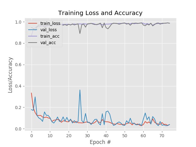
plt.savefig(args["plot"])模型训练:
python train.py -d ./dataset/ -m ./output/keras_model.model \
                -l ./output/keras_labelbin.pickle -p ./output/keras_plot.png
训练 75 个 epoch 的结果为:
loss: 0.0439 - acc: 0.9861 - val_loss: 0.0383 - val_acc: 0.9869
训练过程:
2.5 Multi-label 分类器测试
模型训练后,测试对于新图片的效果 - classifier.py.
from keras.preprocessing.image import img_to_array
from keras.models import load_model
import numpy as np
import argparse
import imutils
import pickle
import cv2
import os
# 设置参数
ap = argparse.ArgumentParser()
ap.add_argument("-m", "--model", required=True,
help="path to trained model model")
ap.add_argument("-l", "--labelbin", required=True,
help="path to label binarizer")
ap.add_argument("-i", "--image", required=True,
help="path to input image")
args = vars(ap.parse_args())
# 加载图片
image = cv2.imread(args["image"])
output = imutils.resize(image, width=400)
# 预处理图片
image = cv2.resize(image, (96, 96))
image = image.astype("float") / 255.0
image = img_to_array(image)
image = np.expand_dims(image, axis=0)
# 加载 CNN 模型和 multi-label binarizer
print("[INFO] loading network...")
model = load_model(args["model"])
mlb = pickle.loads(open(args["labelbin"], "rb").read())
# 图片分类,并找出最大概率的两个类别标签的索引
print("[INFO] classifying image...")
proba = model.predict(image)[0]
idxs = np.argsort(proba)[::-1][:2]
# 对高置信度的类别标签的索引进行循环
for (i, j) in enumerate(idxs):
# 在图片上表示预测的标签
label = "{}: {:.2f}%".format(mlb.classes_[j], proba[j] * 100)
cv2.putText(output, label, (10, (i * 30) + 25),
cv2.FONT_HERSHEY_SIMPLEX, 0.7, (0, 255, 0), 2)
# 分别显示每个独立类别标签的概率
for (label, p) in zip(mlb.classes_, proba):
print("{}: {:.2f}%".format(label, p * 100))
# 显示结果
cv2.imshow("Output", output)
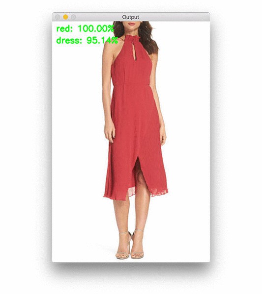
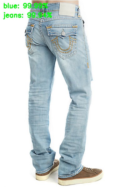
cv2.waitKey(0)图片测试:
python classify.py --model fashion.model \
                    --labelbin ./output/keras_labelbin.pickle \
                    --image examples/example_01.jpg
#
python classify.py --model ./outputkeras_model.model \
                    --labelbin ./output/keras_labelbin.pickle
                    --image examples/example_01.jpg
结果如下:
black: 0.00%
blue: 99.98%
dress: 100.00%
jeans: 0.00%
red: 0.09%
shirt: 0.00%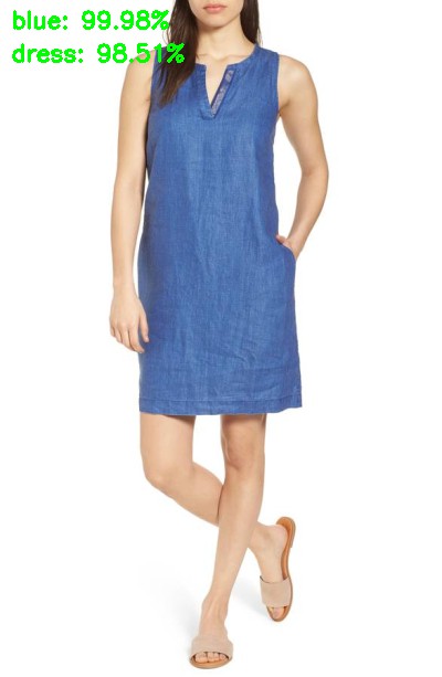
3. 总结
基于 Keras 进行 Multi-label 分类是比较直接简单的,主要包括两步:
- [1] - 替换网络的 softmax 为 sigmoid 激活函数
- [2] - 替换 categorical cross-entropy 损失函数为 binary cross-entropy 损失函数.
实现了一次 forward 同时预测多个类别标签的分类器.
但是,还有一些需要考虑的问题.
需要有待预测类别的每个组合的训练数据(training data for each combination of categories). CNNs 无法预测其没有学习到的多个类别标签组合. 这是因为,网络内部的激活神经元的作用.
例如,如果网络训练是在 "black pant" 和 "red shits" 数据集,但想预测 "red pants" (训练数据不包含 "red pants"),那么检测 "red" 和 "pants" 的网络神经元则会发生变化. 但,由于网络从没有学习到这种组合,一旦它们到了全连接层,预测的结果很有可能不正确.(可能会出现 "red" 或 "pants",但不太可能同时出现 "red" 和 "pants").
故,再次说明,网络很难正确预测其没有被训练过的数据.