原文:Image Segmentation with Tensorflow using CNNs and Conditional Random Fields - 2016.12.18
介绍基于 TF-Slim 库和预训练模型如何实现图像语义分割. 包括模型训练和 CRF(Conditional Random Fiels) 后处理.
1. 介绍
曾介绍过上采样的实现,并通过与 scikit-image 库 中的实现进行对比,以确保实现的正确性. 更具体来说,实现了在论文 Fully convolutional networks for semantic segmentation 中关于 FCN-32 分割网络的实现.
这里,将介绍一种简单的训练:从 PASCAL VOC 数据集随机采样一张图片和对应的标注,在数据集上训练网络,以及在同样的数据集图片测试网络. 这样就也可以在 CPU 上进行模型训练 - 只需要训练 10 次迭代即可完成.
这里还为了说明 FCN-32s 的分割结果是非常粗糙的 - 即使在同样的训练图片上进行分割,结果也是不够很精确的. 此外,还采用了 CRF 对 CNNs 分割结果进行了后处理,通过考虑图像的 RGB 特征和 CNNs 的预测概率来提升分割效果. 最终,得到改善后的图像语义分割结果.
这里,有针对性的简化了训练设置,主要用于说明 FCN-32s 模型的局限性.
类似的方法描述参考论文: Semantic Image Segmentation with Deep Convolutional Nets and Fully Connected CRFs. 采用 Jupyter notebook,可以在每一步可视化代码结果.
image\_segmentation\_conditional\_random\_fields.ipynb
2. 上采样函数和图像加载
环境:
- Tensorflow, TF-Slim
- scikit-image
- numpy 等
在 VGG-16 网络中,max-pooling 层的原因生成降采样的预测结果. 因此,需要进行上采样处理.
另外,还实现了图像和对应的 ground-truth 分割标注的加载函数.
2.1. get_kernel_size 函数
# Upsampling
import numpy as np

def get_kernel_size(factor):
    """
    Find the kernel size given the desired factor of upsampling.
    给定所需的上采样因子,确定卷积核的大小
    """
    return 2 * factor - factor % 2
2.2. upsample_filt 函数
def upsample_filt(size):
    """
    Make a 2D bilinear kernel suitable for upsampling of the given (h, w) size.
    创建一个给定 (h, w) 大小且适用于上采样过程的二维双线性卷积核
    """
    factor = (size + 1) // 2
    if size % 2 == 1:
        center = factor - 1
    else:
        center = factor - 0.5
    og = np.ogrid[:size, :size]
    return (1 - abs(og[0] - center) / factor) * (1 - abs(og[1] - center) / factor)
2.3. bilinear_upsample_weights 函数
def bilinear_upsample_weights(factor, number_of_classes):
    """
    Create weights matrix for transposed convolution with bilinear filter initialization.
    使用双线性滤波器初始化为转置卷积创建权重矩阵
    """

    filter_size = get_kernel_size(factor)

    weights = np.zeros((filter_size,
                        filter_size,
                        number_of_classes,
                        number_of_classes), dtype=np.float32)

    upsample_kernel = upsample_filt(filter_size)

    for i in xrange(number_of_classes):
        weights[:, :, i, i] = upsample_kernel

    return weights
2.4. 数据加载
# Data Loading
from __future__ import division

import os
import sys
import tensorflow as tf
import skimage.io as io
import numpy as np

os.environ["CUDA_VISIBLE_DEVICES"] = '1'
sys.path.append("/home/dpakhom1/workspace/my_models/slim/")
checkpoints_dir = '/home/dpakhom1/checkpoints'

image_filename = 'cat.jpg'
annotation_filename = 'cat_annotation.png'

image_filename_placeholder = tf.placeholder(tf.string)
annotation_filename_placeholder = tf.placeholder(tf.string)
is_training_placeholder = tf.placeholder(tf.bool)

feed_dict_to_use = {image_filename_placeholder: image_filename,
                    annotation_filename_placeholder: annotation_filename,
                    is_training_placeholder: True}

image_tensor = tf.read_file(image_filename_placeholder)
annotation_tensor = tf.read_file(annotation_filename_placeholder)

image_tensor = tf.image.decode_jpeg(image_tensor, channels=3)
annotation_tensor = tf.image.decode_png(annotation_tensor, channels=1)

# 对于每个类别,将其设置为1而不是一个数字 -- 用于计算交叉熵损失函数.
# 实际中,groundtruth masks 还包含除了 1 和 0 的其它值.
class_labels_tensor = tf.equal(annotation_tensor, 1)
background_labels_tensor = tf.not_equal(annotation_tensor, 1)

# 将布尔值转换为浮点数 -- 用于正确计算交叉熵 loss
bit_mask_class = tf.to_float(class_labels_tensor)
bit_mask_background = tf.to_float(background_labels_tensor)

combined_mask = tf.concat(concat_dim=2, values=[bit_mask_class,
                                                bit_mask_background])

# 调整输入数据的大小,
# 保持与 tf.softmax_cross_entropy_with_logits 的 [batch_size, num_classes] 尺寸相一致.
flat_labels = tf.reshape(tensor=combined_mask, shape=(-1, 2))
3. loss 函数和 Adam 模型训练
这里,添加上采样层到网络,定义可微的 loss 函数,然后进行训练.
根据论文 Fully convolutional networks for semantic segmentation,定义 loss 函数为像素级交叉熵函数.
在上采样后,可以得到与输入图像尺寸一致的预测结果,分割结果与对应的 groundtruth 分割标注的 loss 计算为:
此时,可以采用 Adam 优化算法进行学习,因为其具有更少的参数,并能得到比较好的结果. 以在一张图像上进行模型训练和评估的特殊情况为例 - 相对于真实训练场景而言,这种训练方式很简单. 目的只是为了表明方法的不足 - 较差的定位能力. 换句话说,如果在这样的简单情况下,得到的结果很差,那么在未训练的图像上,其结果会更差.
import numpy as np
import tensorflow as tf
import sys
import os
from matplotlib import pyplot as plt
fig_size = [15, 4]
plt.rcParams["figure.figsize"] = fig_size
import urllib2
slim = tf.contrib.slim
from nets import vgg
from preprocessing import vgg_preprocessing
# 均值加载,减均值函数加载
from preprocessing.vgg_preprocessing import (
_mean_image_subtraction,_R_MEAN, _G_MEAN, _B_MEAN)
upsample_factor = 32
number_of_classes = 2
log_folder = '/home/dpakhom1/tf_projects/segmentation/log_folder'
vgg_checkpoint_path = os.path.join(checkpoints_dir, 'vgg_16.ckpt')
# 图像减均值前,先转换为 float32 数据类型
image_float = tf.to_float(image_tensor, name='ToFloat')
# 每个像素进行减均值
mean_centered_image = _mean_image_subtraction(
image_float, [_R_MEAN, _G_MEAN, _B_MEAN])
processed_images = tf.expand_dims(mean_centered_image, 0)
upsample_filter_np = bilinear_upsample_weights(upsample_factor, number_of_classes)
upsample_filter_tensor = tf.constant(upsample_filter_np)
# 模型定义 -- 最后一层输出层仅有 2 个类别.
with slim.arg_scope(vgg.vgg_arg_scope()):
logits, end_points = vgg.vgg_16(processed_images,
num_classes=2, #
is_training=is_training_placeholder,
spatial_squeeze=False,
fc_conv_padding='SAME')
downsampled_logits_shape = tf.shape(logits)
# 计算上采样 tensor 的输出尺寸
upsampled_logits_shape = tf.pack([
downsampled_logits_shape[0],
downsampled_logits_shape[1] * upsample_factor,
downsampled_logits_shape[2] * upsample_factor,
downsampled_logits_shape[3]
])
# 上采样处理 upsampling
upsampled_logits = tf.nn.conv2d_transpose(
logits,
upsample_filter_tensor,
output_shape=upsampled_logits_shape,
strides=[1, upsample_factor, upsample_factor, 1])
# 展开预测结果,以计算每个像素的交叉熵损失,得到交叉熵总和.
flat_logits = tf.reshape(tensor=upsampled_logits,
shape=(-1, number_of_classes))
cross_entropies = tf.nn.softmax_cross_entropy_with_logits(
logits=flat_logits, labels=flat_labels)
cross_entropy_sum = tf.reduce_sum(cross_entropies)
# 每个像素最终的预测结果 Tensor
# 不需要计算 softmax,因为只是需要最终的决策.
# 如果需要各个类别的概率,则必须进行 softmax.
pred = tf.argmax(upsampled_logits, dimension=3)
probabilities = tf.nn.softmax(upsampled_logits)
# 定义优化器,添加所有将创建到 `adam_vars` 命名空间的变量.
# 便于有效的变量访问.
# 添加的变量供给 adam 优化器使用,且与 VGG 模型的变量不相关.
# 另外,还计算了每个变量的梯度 Tensors. 用于 tensorboard 中的可视化.
# optimizer.compute_gradients 和 optimizer.apply_gradients 等价于:
# train_step = tf.train.AdamOptimizer(learning_rate=0.0001).minimize(cross_entropy_sum)
with tf.variable_scope("adam_vars"):
optimizer = tf.train.AdamOptimizer(learning_rate=0.0001)
gradients = optimizer.compute_gradients(loss=cross_entropy_sum)
for grad_var_pair in gradients:
current_variable = grad_var_pair[1]
current_gradient = grad_var_pair[0]
# 替换原始变量名中的某些字符,如:tensorboard 不支持 ':' 符号.
gradient_name_to_save = current_variable.name.replace(":", "_")
# 计算每一层的梯度直方图,以在 tensorboard 中进行了可视化.
tf.summary.histogram(gradient_name_to_save, current_gradient)
train_step = optimizer.apply_gradients(grads_and_vars=gradients)
# 定义一个函数,用于加载 VGG 断点中的权重数据,加载到变量.
# 去除最后一层用于预测类别的权重. 因为类别数不相同.
vgg_except_fc8_weights = slim.get_variables_to_restore(exclude=['vgg_16/fc8', 'adam_vars'])
# 得到网络最后一层的权重变量.
# VGG 网络的类别数与定义的网络是不相同的,这里只有 2 类.
vgg_fc8_weights = slim.get_variables_to_restore(include=['vgg_16/fc8'])
adam_optimizer_variables = slim.get_variables_to_restore(include=['adam_vars'])
# 为 loss 添加 summary op,用于在 tensorboard 中的可视化.
tf.summary.scalar('cross_entropy_loss', cross_entropy_sum)
# 合并所有的 summary ops 为一个 op.
# 运行时生成字符串
merged_summary_op = tf.summary.merge_all()
# 创建 summary writer -- 将 log 写入指定文件,用于 tensorboard 的读取.
summary_string_writer = tf.summary.FileWriter(log_folder)
# 创建 log 保存路径
if not os.path.exists(log_folder):
os.makedirs(log_folder)
# 创建 OP,以对变量值初始化为从 VGG 加载的值.
read_vgg_weights_except_fc8_func = slim.assign_from_checkpoint_fn(
vgg_checkpoint_path,
vgg_except_fc8_weights)
# 对 fc8 weights 进行权重初始化 -- for two classes.
vgg_fc8_weights_initializer = tf.variables_initializer(vgg_fc8_weights)
# adam 变量的初始化
optimization_variables_initializer = tf.variables_initializer(adam_optimizer_variables)
with tf.Session() as sess:
# 运行初始化
read_vgg_weights_except_fc8_func(sess)
sess.run(vgg_fc8_weights_initializer)
sess.run(optimization_variables_initializer)
train_image, train_annotation = sess.run([
image_tensor, annotation_tensor],
feed_dict=feed_dict_to_use)
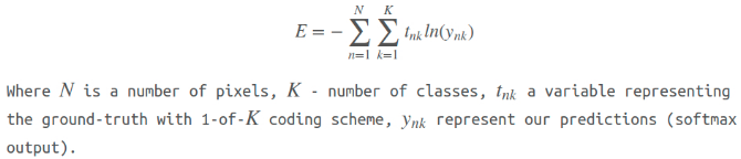
f, (ax1, ax2) = plt.subplots(1, 2, sharey=True)
ax1.imshow(train_image)
ax1.set_title('Input image')
probability_graph = ax2.imshow(np.dstack((train_annotation,)*3)*100)
ax2.set_title('Input Ground-Truth Annotation')
plt.show()
# 运行 10 次迭代.
for i in range(10):
loss, summary_string = sess.run(
[cross_entropy_sum, merged_summary_op],
feed_dict=feed_dict_to_use)
sess.run(train_step, feed_dict=feed_dict_to_use)
pred_np, probabilities_np = sess.run(
[pred, probabilities],
feed_dict=feed_dict_to_use)
summary_string_writer.add_summary(summary_string, i)
cmap = plt.get_cmap('bwr')
f, (ax1, ax2) = plt.subplots(1, 2, sharey=True)
ax1.imshow(np.uint8(pred_np.squeeze() != 1), vmax=1.5, vmin=-0.4, cmap=cmap)
ax1.set_title('Argmax. Iteration # ' + str(i))
probability_graph = ax2.imshow(probabilities_np.squeeze()[:, :, 0])
ax2.set_title('Probability of the Class. Iteration # ' + str(i))
plt.colorbar(probability_graph)
plt.show()
print("Current Loss: " + str(loss))
feed_dict_to_use[is_training_placeholder] = False
final_predictions, final_probabilities, final_loss = \
sess.run([pred,probabilities,cross_entropy_sum],
feed_dict=feed_dict_to_use)
f, (ax1, ax2) = plt.subplots(1, 2, sharey=True)
ax1.imshow(np.uint8(final_predictions.squeeze() != 1),
vmax=1.5,
vmin=-0.4,
cmap=cmap)
ax1.set_title('Final Argmax')
probability_graph = ax2.imshow(final_probabilities.squeeze()[:, :, 0])
ax2.set_title('Final Probability of the Class')
plt.colorbar(probability_graph)
plt.show()
print("Final Loss: " + str(final_loss))
summary_string_writer.close()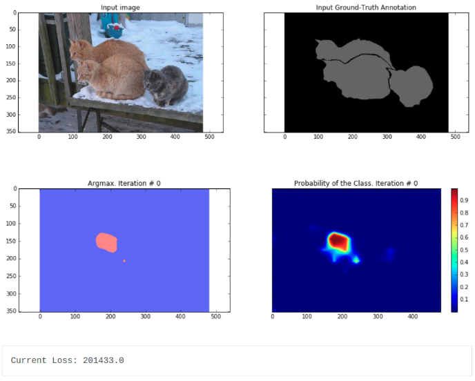
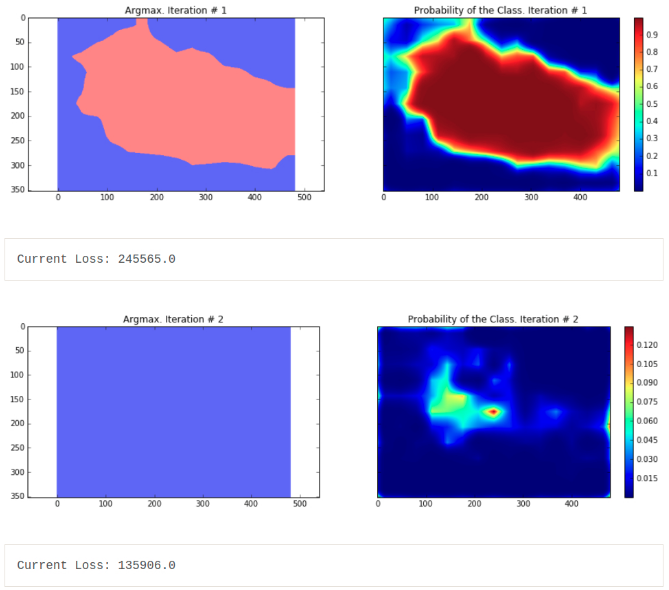
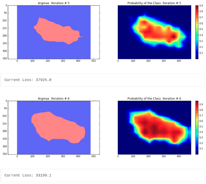
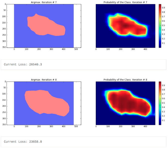

可以看出,分割的结果非常粗糙 - 这些结果是由在相同训练图片上训练的模型输出的结果.
分割中是常见问题,分割结果通常很粗糙. 有很多方法来改善这样的问题,比如采用跳跃链接. 跳跃链接的主要思想是,融合网络不同层的预测结果. 由于在网络靠前的层中,下采样因子比较小,更易于定位. 详细可见论文 Fully convolutional networks for semantic segmentation. 其中,还给出了 FCN-16s 和 FCN-8s 网络结构.
另一种方法是,采用 atrous convolutions 和全连接CRFs(fully connected conditional random fields). 可见论文:Semantic Image Segmentation with Deep Convolutional Nets and Fully Connected CRFs.
下面只采用 CRF 后处理方法,提升语义分割结果. 此外,这里训练模型时,采用了 dropout 技术(Dropout: a simple way to prevent neural networks from overfitting). Dropout 是用于模型训练的正则化技术,其理论优秀,且实现简单:只需在每个训练迭代中,随机选择一部分神经元,进行网络学习和后向传播. 理论方面,Dropout可以看作是通过权重共享来训练一个稀疏网络的集合,每个网络仅进行很少的训练. 测试时,对这些网络所有的预测结果进行求平均. 论文中说明了,对于线性回归, Dropout 预期能够取得类似于岭回归的效果. 在这里,仅将 Dropout 用于全连接层(映射到卷积层的全连接层). 这也解释了最终模型的损失基本上比最后一次迭代小了两倍的原因 - 模型最后推断的损失使用了均值. 上面的长代码用于单张图像的,但能够很容易的用于整个数据集. 只需要调整每次迭代中输入的图像. 参考论文:Fully convolutional networks for semantic segmentation. FCNs 的分割结果仍比较粗糙,需要进行进一步的后处理. 比如 FC-CRFs,以精细化分割粒度.
4. CRFs 后处理
CRFs 是图模型的一种特定形式. 这里其有助于在给定网络预测结果和原始图像的 RGB 特征时,估计模型预测结果的后验分布. 通过对用户定义的能量函数的最小化来实现. 在这里,其类似于双边滤波器(bilateral filter)的效果. 双边滤波器同时考虑了图像中像素的空间临近性和 RGB 特征空间(强度空间)相似性. 简单来说,CRFs 采用 RGB 特征以使得图像分割精度更高 - 如,边界通常表示为大的强度变化 - 这是一个关键因素,位于该边界两侧的物体分别属于不同的类别. 另外,CRFs 也对小分割区域进行惩罚 - 如,20 pixels 或 50 pixels 的分割区域通常不是正确的分割区域. 物体通常表示为大的空间临近区域. 下面使用 CRFs 后处理来进一步处理分割结果. 参考了论文 fully connected crfs with gaussian edge potentials
import sys

path = "/home/dpakhom1/dense_crf_python/"
sys.path.append(path)

import pydensecrf.densecrf as dcrf

from pydensecrf.utils import compute_unary, create_pairwise_bilateral, \
    create_pairwise_gaussian, softmax_to_unary

import skimage.io as io

image = train_image
softmax = final_probabilities.squeeze()
softmax = processed_probabilities.transpose((2, 0, 1))

# softmax_to_unary函数的输入数据为概率值的负对数
unary = softmax_to_unary(processed_probabilities)

# 输入数据应该是 C-continious -- 这里采用 Cython 封装器
unary = np.ascontiguousarray(unary)

d = dcrf.DenseCRF(image.shape[0] * image.shape[1], 2)

d.setUnaryEnergy(unary)

# 对空间独立的小分割区域进行潜在地惩罚 - 促使生成更多连续的分割区域.
feats = create_pairwise_gaussian(sdims=(10, 10), shape=image.shape[:2])

d.addPairwiseEnergy(feats, compat=3,
                    kernel=dcrf.DIAG_KERNEL,
                    normalization=dcrf.NORMALIZE_SYMMETRIC)

# 创建与颜色相关的特征
# 因为 CNN 的分割结果太粗糙,使用局部的颜色特征来进一步提升分割结果.
feats = create_pairwise_bilateral(sdims=(50, 50), schan=(20, 20, 20),
                                   img=image, chdim=2)

d.addPairwiseEnergy(feats, compat=10,
                     kernel=dcrf.DIAG_KERNEL,
                     normalization=dcrf.NORMALIZE_SYMMETRIC)
Q = d.inference(5)

res = np.argmax(Q, axis=0).reshape((image.shape[0], image.shape[1]))

cmap = plt.get_cmap('bwr')

f, (ax1, ax2) = plt.subplots(1, 2, sharey=True)
ax1.imshow(res, vmax=1.5, vmin=-0.4, cmap=cmap)
ax1.set_title('Segmentation with CRF post-processing')
probability_graph = ax2.imshow(np.dstack((train_annotation,)*3)*100)
ax2.set_title('Ground-Truth Annotation')
plt.show()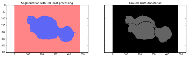
5. 总结和讨论
这里主要介绍了 CNN 进行图像语义分割的一个局限性 - 粗糙的分割结果.
可以看出,这是由于 VGG-16 网络中的 max pooling 层导致的. 针对简单情况进行模型训练,定义损失函数为像素级交叉熵损失,采用后向传播更新权重.
另外,采用 CRFs 进一步改进语义分割结果粗糙的问题,取得了较好的效果.
24 条评论
您好,请问我输入原图像为rgb图像,预测图像为二值图,使用crf之后的结果全黑,可能的原因是什么?
二值图貌似 crf 出来结果确实是全黑的,你把二值图换成概率图试试.
我想请问下,我的原始图片是二维图片并且是二分类,怎么用CRF来进行优化呢?
还有image=train_image指的是原RGB用来分割的图 ,但原文就是个变量 我要改成RGB图的路径么还是写成什么格式
crf 只有后处理,跟 CNN 网络计算过程部分无关,crf 输入就是原始 RGB 图片和 CNN 网络所输出的概率图.
概率图是那个分割图么 还是经过最后一层卷积 sigmoid最后输出的output_4 如果是这个output_4的话 那怎么将其导入到CRF的Py文件中
对啊,直接 imread 读入.
楼主 CRFS后处理那段 我下载了fully connected CRFs 库 那是不是只要对于最后那段代码稍加修改我就可以将我的分割粗糙图精修出来 无需和前文代码更多的联系
CRF 只是后处理的一种处理,效果不一定是能够将粗糙图精修;代码实现是不需要与前文代码有多少联系.
楼主 CRF代码中第13行image = train_image指的是训练集的Image还是我分割出来的粗糙image
原始 RGB 图片.
楼主有很多问题又来麻烦你了
softmax = final_probabilities.squeeze()
softmax = processed_probabilities.transpose((2, 0, 1))
final_probabilities.squeeze()和 processed_probabilities.transpose 原文中没被定义啊
final_probabilities 就是语义分割网络的输出结果.
前文中实在没找到processed_probabilities.transpose 不知何意 麻烦了博主
这两个作用都是一样的,取一个就行了,就是 CNN 的输出.
原文中path路径指的什么 是指我网络输出的Py文件的路径么
那 processed_probabilities.transpose 呢
请问您解决这个问题了吗 我也好疑惑啊
博主 遇到好多问题 实在麻烦你了1. 原文CRF那个是单独的py文件么?是否可以单独运行不管我的model和train文件?
毕竟我已经分割出了很不错的图 只是需要精修
我也是需要边缘精修,请问您现在解决这个问题了吗(ó﹏ò。)
如何不是单独运行 那是要写在哪 是写在我自己分割网络输出所在的def函数中么?
最后这段程序好像不对,
希望您可以提供解答
不对是指?