原文 - Tips for building fast portrait segmentation network with TensorFlow Lite 主要是 TensorFLow Lite 上的速度优化技巧.

<h2>前言</h2>

深度学习在很多领域取得了一系列的突破. 但，深度学习模型一般需要很多的计算资源，内存和计算力.
深度模型在移动设备上的部署，对于很多移动科技公司来说，成为主要的技术挑战.

Hyperconnect 开发了一款名为 Azar 的移动应用，在世界上有很多用户.
最近，其机器学习团队专注于开发移动深度学习技术，以提升 Azar 的用户体验.
下面的例示给出了采用图像语义分割技术(HyperCut)的 demo，基于 Samsung Galaxy J7. 该项目的基准目标是，采用单核在 Galaxy J7 (Exynos 7580 CPU, 1.5 GHz) 上实时推断(>=30 fps).

Figure 1. 移动设备上网络的快速运行示例. 在 Pixel 1 上可以达到单次推断 6ms；在 Galaxy J7 上单次推断 28 ms. 完整 Video.

移动设备上快速推断的实现有几种不同的方法. 8-bit quantization，是一种能够满足项目的速度-精度要求的常用方法.
采用 TensorFlow Lite 作为移动推断的深度框架. TensorFlow Lite 支持对 8-bit 权重和激活值的 SIMD 优化操作. 但是，TensorFlow Lite 仍处于 pre-alpha 阶段，缺乏很多特征.
因此，为了达到项目目标，主要进行工作如下：

• [1] - 理解 TensorFlow 和 TensorFlow Lite 的实现细节
• [2] - 设计神经网络，充分利用 TensorFlow Lite 的 optimized kernels (参考章节 1, 2, 3).
• [3] - 修改 TOCO: TensorFlow Lite Optimizing Converter 以正确转换未支持的网络层(参考章节 4).
• [4] - 采用 SIMD 优化代码，加速 quantized-layers (参考章节 5, 6).

这里对项目过程中进行的尝试和遇到的错误进行分享，以供开发移动深度模型.

<h2>1. Tensorflow Lite 中的深度可分离层(depthwise separable layer) 为什么速度快？</h2>

low-level programs 的实现需要一些不同的思想和方法.
尤其是在采用 cache memory 的移动设备上的编程，快速推断更是重要.

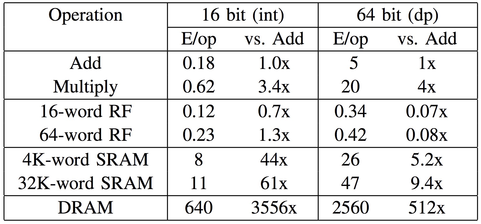
Figure 2. 内存访问比加法或乘法需要更多的资源(640 pJ). 访问 cache memory (8 pJ) 比使用 main memory 资源占用少很多.[图片来自 Ardavan Pedram]

为了深入 TensorFlow Lite 中的实现，需要分析一些具体实现，例如 depthwise separable convolution with 3x3 kernels.

下面介绍用于构建轻量和快速编程采用的几种主要优化技术.

<h3>1.1 Loop Unrolling</h3>

比较如下两种代码实现的不同：
风格1：

for (int i = 0; i < 32; i++) {
  x[i] = 1;
  if (i%4 == 3) x[i] = 3;
}

风格2：

for (int i = 0; i < 8; i++) {
  x[4*i  ] = 1;
  x[4*i+1] = 1;
  x[4*i+2] = 1;
  x[4*i+3] = 3;
}

第一种代码风格是比较常用的，第二种风格是 loop-unrolled 版.
即使 unrolling loops 由于代码冗余问题，在软件设计和开发中被舍弃，但在 low-level 结构中，其有不可忽略的优点.
例如上面代码，unrolled 风格的代码，避免了 for 循环中的 24 次条件判断，且少了 32 次 if 条件判断.

此外，采用 SIMD 结构，可以进一步提升 unrolling loops 的优势.
现在有一些编译器已经支持自动 unrool 一些重复代码语句，但仍难以处理复杂 loops .

<h3>1.2 Separate implementation for each case</h3>

卷积层包含了几个参数. 例如，在深度可分离层(depthwise separable layer)中，有很多不同参数的组合(depth_multiplier x stride x rate x kernel_size).
在 low-level 编程中，定义多个特定情况的实现，要比采用适用于每个情况的单行编程，更有优势.
其基本原理是，充分利用每种情况的属性特点(need to fully utilize the special properties for each case).
对于卷积操作，其初级实现是，采用几个 for loops 来处理任意 kernel size 和 strides，但是，这种实现的速度可能会慢一些.
相反，可以采用针对具体情况的轻量实现(如，stride=1 的 1x1 conv，stride=2的 3x3 conv，等等)，充分考虑每个子问题的结构.

例如， 在 TensorFlow Lite 中，depthwise convolution 的 kernel-optimized 实现，用于 3x3 kernel：

template <int kFixedOutputY, int kFixedOutputX, int kFixedStrideWidth, int kFixedStrideHeight>
struct ConvKernel3x3FilterDepth8 {};

TensorFlow Lite 进一步指定了不同 strides，输出width 和 height 的 16 种情况的实现，

template <> struct ConvKernel3x3FilterDepth8<8, 8, 1, 1> { ... }
template <> struct ConvKernel3x3FilterDepth8<4, 4, 1, 1> { ... }
template <> struct ConvKernel3x3FilterDepth8<4, 2, 1, 1> { ... }
template <> struct ConvKernel3x3FilterDepth8<4, 1, 1, 1> { ... }
template <> struct ConvKernel3x3FilterDepth8<2, 2, 1, 1> { ... }
template <> struct ConvKernel3x3FilterDepth8<2, 4, 1, 1> { ... }
template <> struct ConvKernel3x3FilterDepth8<1, 4, 1, 1> { ... }
template <> struct ConvKernel3x3FilterDepth8<2, 1, 1, 1> { ... }
template <> struct ConvKernel3x3FilterDepth8<4, 2, 2, 2> { ... }
template <> struct ConvKernel3x3FilterDepth8<4, 4, 2, 2> { ... }
template <> struct ConvKernel3x3FilterDepth8<4, 1, 2, 2> { ... }
template <> struct ConvKernel3x3FilterDepth8<2, 2, 2, 2> { ... }
template <> struct ConvKernel3x3FilterDepth8<2, 4, 2, 2> { ... }
template <> struct ConvKernel3x3FilterDepth8<2, 1, 2, 2> { ... }
template <> struct ConvKernel3x3FilterDepth8<1, 2, 2, 2> { ... }
template <> struct ConvKernel3x3FilterDepth8<1, 4, 2, 2> { ... }

<h3>1.3 智能内存访问模式 Smart Memory Access Pattern</h3>

由于 low-level 编程是以重复的模式执行很多次，最小化输入和输出的重复内存访问很有必要.
如果采用 SIMD 结构，可以一次加载临近元素(Data Parallelism)；而且，为了减少重复的内存读访问，可以以 snake-path 方式穿过输入数组(input array)：

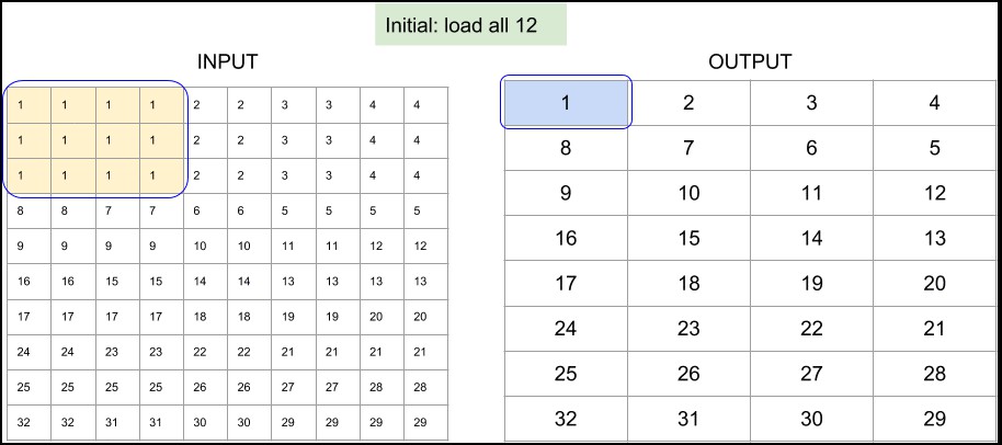
Figure 3. TensorFlow Lite 的 depthwise 3x3 conv 实现中，8x8 输出和单位步长的内存访问模式.

下面的例子，用于在更小的 4x1 输出块，也示例了如何有效的重用预加载变量.
其中，用于保存先前阶段加载的变量的位置不发生变化.

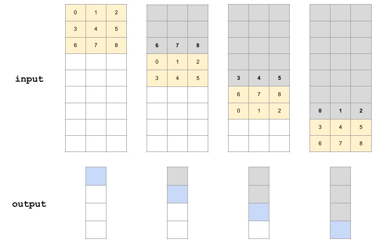
Figure 4. TensorFlow Lite 的 depthwise 3x3 conv 实现中，4x1 输出和步长为2的内存访问模式.(加粗变量被重用)

<h2>2. atrous depthwise convolution 的理解</h2>

Atrous Conv 对于图像分割很有帮助. 该项目也会应用到.
有次，当尝试设置 atrous depthwise convolution 的步长来计算计算时，由于 TensorFLow(<=1.8) 中网络层的限制，并未成功.

在 TensorFlow 的 tf.nn.depthwise_conv2d 文档中，(slim.depthwise_conv2d 也封装了该函数)，可以找到关于 rate 参数的解释：

rate: 1-D of size 2. 
The dilation rate in which we sample input values across the height and width dimensions in atrous convolution. 
If it is greater than 1, then all values of strides must be 1.

即使 TensorFlow 不支持不同步长的 atrous 函数，但设置 rate>1 和 stride>1 进行运行时，也不会出现任何错误提示.

>>> import tensorflow as tf
>>> tf.enable_eager_execution()
>>> input_tensor = tf.constant(list(range(64)), shape=[1, 8, 8, 1], dtype=tf.float32)
>>> filter_tensor = tf.constant(list(range(1, 10)), shape=[3, 3, 1, 1], dtype=tf.float32)
>>> print(tf.nn.depthwise_conv2d(input_tensor, filter_tensor,
                                 strides=[1, 2, 2, 1], padding="VALID", rate=[2, 2]))

tf.Tensor(
[[[[ 302.] [ 330.] [ 548.] [ 587.]]
  [[ 526.] [ 554.] [ 860.] [ 899.]]
  [[1284.] [1317.] [1920.] [1965.]]
  [[1548.] [1581.] [2280.] [2325.]]]], shape=(1, 4, 4, 1), dtype=float32)

>>> 0  5 + 2  6 + 16  8 + 9  18   # The value in (0, 0) is correct
302
>>> 0  4 + 2  5 + 4  6 + 16  7 + 18  8 + 20  9   # But, the value in (0, 1) is wrong!
470

这里分析其原因.

如果只在卷积层前后放置 tf.space_to_batch 和 tf.space_to_batch，则可以采用 atrous conv 的卷积操作.
另一方面，对于如何一起使用 stride 和 dilation ，并未直接给出.
在 TensorFlow 中，需要知道 depthwise conv 的这个问题.

<h2>3. 高效语义分割网络的设计原则</h2>

通常情况下，语义分割比图像分类需要耗费更多时间，因为其需要上采样到高分辨率(hifh spatial resolution map).
因此，尽可能减少推断时间，以实时预测，甚为重要.

在设计实时应用时，空间分辨率需要着重关注. 最简单的方式是，在不损失精度的前提下，减少输入图像的尺寸. 假设网络是全卷积的，如果输入图像的尺寸减半，则可以将模型速度提高 4 倍. 论文 [Rethinking the Inception Architecture for Computer Vision] 中，说明了小尺寸的输入图片不会影响太多精度.

另外一种简单策略是，当堆积卷积层时，进行下采样. 即使是相同数量的卷积层，采用 strided conv 或 pooling，也可以减少运行时间.

使用 TensorFlow Lite 量化模型时，输入图像尺寸的选取有一个技巧. 当图像的 width 和 height 是 8 的倍数时，卷积操作可以运行最快.
Tensorflow Lite 首先加载 8 的倍数，然后分别是 4, 2 和 1 的倍数. 因此，最佳的是，保持卷积层的每个输入的尺寸为 8 的倍数.

将多个操作替换为单个操作，也可以提升一点速度. 例如，conv + max pooling 通常可以替换为 strided conv. Transpose conv 也可以替换为 resizing + conv. 一般情况下，这些操作可以进行替换的原因是其在网络中的作用相同. 并没有大的差异.

以上技巧可以提升推断速度，但也会损失精度. 因此，该项目采用新的网络块，而不是原本的卷积块.

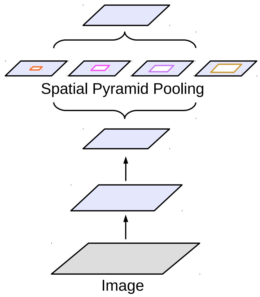
Figure 5. Atrous spatial pyramid pooling, ASPP

ASPP 整合了 pyramid pooling 和 atrous conv 操作. DeepLab 在最后一层采用了 ASPP.

该项目替换了大部分 conv 层为 depthwise separable convolution 层. depthwise separable convolution 层是 MobileNetV1 和 MobileNetV2 的基础构建模块，其在 Tensorflow Lite 中进行了很好的优化.

<h2>4. 将 batchnorm 折叠进 atrous depthwise convolution</h2>

当在 conv 操作后采用 batchnorm 时，batchnorm 层必须折叠进 conv 层，以减少计算耗费.
折叠后，batchnorm 减少为折叠权重(folded weights)和折叠偏置(folded biases)，折叠 batchnorm 的 conv 操作在 TensorFlow Lite 中可以在单个卷积层进行计算.
如果 batchnorm 层紧接在 conv 层后，采用 tf.contrib.quantize 可以自动折叠 batchnorm.
然而，将 batchnorm 折叠进 atrous depthwise convolution 并不容易.

TensorFlow 的 slim.separable_convolution2d 中，atrous depthwise convolution 的实现是通过将 SpaceToBatchND 和 SpaceToSpaceND 操作添加到 normal depthwise convolution 中.
如果，在添加 batchnorm 时，设置参数 normalizer_fn=slim.batch_norm，batchnorm 并未直接添加到 conv 层. 而是，graph 类似于如下：

SpaceToBatchND → DepthwiseConv2dNative → BatchToSpaceND → BatchNorm

首先尝试的是，修改 TensorFlow 量化来折叠 batchnorm，避开 BatchToSpaceND，而不改变各操作的次序. 这样，BatchToSpaceND 后保留了 folded bias 项，远离 conv 层.
然后，在 TensorFlow Lite 模型中变为 separate BroadcastAdd 操作，而不是融合进 conv.
令人惊奇的是，实验中，BroadcastAdd 比对应的 conv 操作慢了很多.

Timing log from the experiment on Galaxy S8
...
[DepthwiseConv] elapsed time: 34us
[BroadcastAdd]  elapsed time: 107us
...

为了移除 BroadcastAdd 层，该项目修改了网络本身，而不是固定 TensorFLow 量化.
采用 slim.separable_convolution2d 层，调换 BatchNorm 和 BatchToSpaceND 的位置：

SpaceToBatchND → DepthwiseConv2dNative → BatchNorm → BatchToSpaceND

即使调整 batchnorm 位置后，可能会导致不同的输出值. 但并未损失分割质量.

<h2>5. SIMD-optimized implementation for quantized resize bilinear layer</h2>

加速 TensorFlow Lite 框架时，不支持 con2d_transpose 层.
但是，可以采用 ResizeBilinear 层，处理上采样(upsampling). 但问题是，其没有量化实现.
因此，该项目实现了 2x2 上采样 ResizeBilinear 层的 SIMD 量化优化版本.

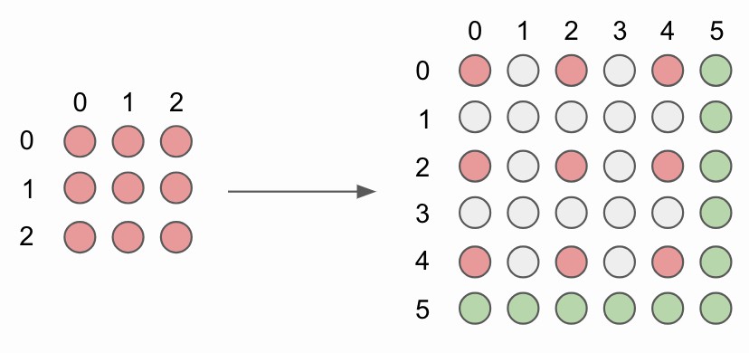
Figure 6. 没有角对齐(corner alignment) 的 2x2 双线性上采样.

为了上采样图像，原始图像像素(红色圈)由新插值的图像像素(灰色圈)隔开.
简单起见，对最下面和最右面的像素不进行计算像素值(绿色圈).

for (int b = 0; b < batches; b++) {
  for (int y0 = 0, y = 0; y <= output_height - 2; y += 2, y0++) {
    for (int x0 = 0, x = 0; x <= output_width - 2; x += 2, x0++) {
      int32 x1 = std::min(x0 + 1, input_width - 1);
      int32 y1 = std::min(y0 + 1, input_height - 1);
      ResizeBilinearKernel2x2(x0, x1, y0, y1, x, y, depth, b, input_data, input_dims, output_data, output_dims);
    }
  }
}

对于每个 batch，分别计算每个新像素的值. 核心函数 ResizeBilinearKernel2x2 一次计算多个通道的 4 个像素值.

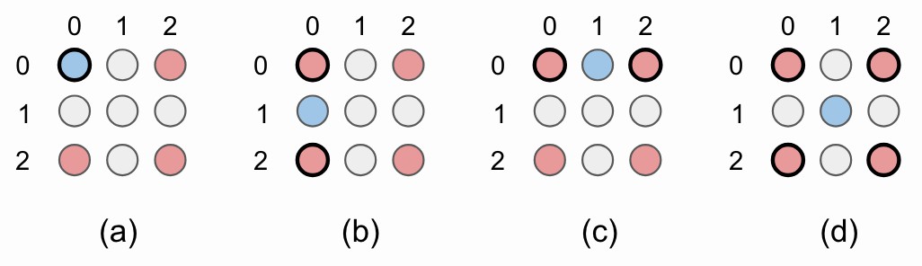
Figure 7. 图像的左上角的 2x2 上采样例示. (a) 原来的像素值被重用；(b)-(d) 用于插值新像素值. 红色圈表示原来的像素值. 蓝色圈是新插值的像素值，由黑色圆圈表示的像素值计算得到.

NEON (Advanced SIMD) intrinsics 可以单指令一次处理多个数据. 由于项目处理的 uint8 输入值，可以保存数据为 uint8x16_t, uint8x8_t 和 uint8_t 格式，分别表示 16, 8 和 1 uint8 值. 这种表示可以一次跨多个通道插值像素值.
当 feature maps 的通道是 16 或 8 的倍数时，这样网络结构十分推荐.

// Handle 16 input channels at once
int step = 16;
for (int ic16 = ic; ic16 <= depth - step; ic16 += step) {
  ...
  ic += step;
}

// Handle 8 input channels at a once
step = 8;
for (int ic8 = ic; ic8 <= depth - step; ic8 += step) {
  ...
  ic += step;
}

// Handle one input channel at once
for (int ic1 = ic; ic1 < depth; ic1++) {
  ...
}

quantized bilinear upsampling 的 SIMD 实现是很直接的. 左上角的像素值被重用(Fig 7a)，左下(Fig 7b) 和右上(Fig 7c) 的像素值是两个原来临近像素值的均值. 最后，右下像素值(Fig 7d) 是 4 个原来对角线临近像素值的均值.

唯一的问题是，必须要注意 8-bit 整数溢出. 由于没有深入理解 NEON intrinsics，因此并未继续溢出问题.
幸运的是， NEON intrinsics 的范围比较广泛，可以用于满足项目需求.
下面的代码片段(使用 vrhaddq_u8) 给出了右下像素值的一次插值 16 个像素值.

// Bottom right
output_ptr += output_x_offset;
uint8x16_t left_interpolation = vrhaddq_u8(x0y0, x0y1);
uint8x16_t right_interpolation = vrhaddq_u8(x1y0, x1y1);
uint8x16_t bottom_right_interpolation = vrhaddq_u8(left_interpolation, right_interpolation);
vst1q_u8(output_ptr, bottom_right_interpolation);

<h2>6. Softmax 层和 demo 代码中易出现的错误</h2>

TensorFlow Lite 推断时的第一印象是比较慢. 在 Galaxy J7 上耗费 85 ms.
测试 TensorFlow Lite demo app 的第一个原型时，只改变了输出尺寸为 1001 到 51200(=160x160x2).

测试后，发现了实现中两个难以置信的瓶颈.
推断时间的 85 ms 中，Tensor.java 中的 tensors[idx].copyTo(outputs.get(idx)); 行占用了 11 ms(13%)，softmax 层占用了 23 ms(27%).
如果能够加速这两处，则能够减少总共推断时间的 40%.

首先，对于 demo 代码中 tensors[idx].copyTo(outputs.get(idx)); 的问题. 其速度慢的原因看起来可能是由 copyTo 操作导致，但实际上却是由 int[] dstShape = NativeInterpreterWrapper.shapeOf(dst); 导致的，因为其检查数组的每个元素(这里是，51200 个). 固定输出尺寸后，推断时间有了 13% 的提升.

<T> T copyTo(T dst) {
  ...
  // This is just example, of course, hardcoding output shape here is a bad practice
  // In our actual app, we build our own JNI interface with just using c++ code
  // int[] dstShape = NativeInterpreterWrapper.shapeOf(dst);
  int[] dstShape = {1, widthheightchannel};
  ...
}

然后，是 Softmax 层的问题. TensorFlow Lite 的 优化的 softmax 实现 假设 depth (= channel) 大于 outer_size (= height x width).
在分类问题中，其输出一般是 [1, 1(height), 1(width), 1001(depth)]. 但是在分割问题中，depth=2，outer_size=height x width(outer_size » depth).

TensorFlow Lite 中 Softmax 层的实现是对分类任务优化的，然后在 depth 上进行循环，而不是 outer_size. 这就会导致在分割网络中使用 softmax 层推断时间较慢.

可以采用很多不同的方法来解决该问题.
第一种，在 2-class 肖像分割中，采用 sigmoid 层，而不是 softmax 层. TensorFlow Lite 中较好的优化了 sigmoid 层.

第二种，采用 SIMD 优化代码，对 depth 进行循环，而不是 outer_size. 可以参考 Tencent 的 ncnn softmax layer. 但是，这种方法仍有缺点，不像 ncnn，TensorFlow Lite 采用 NHWC 作为默认的 tensor 格式：

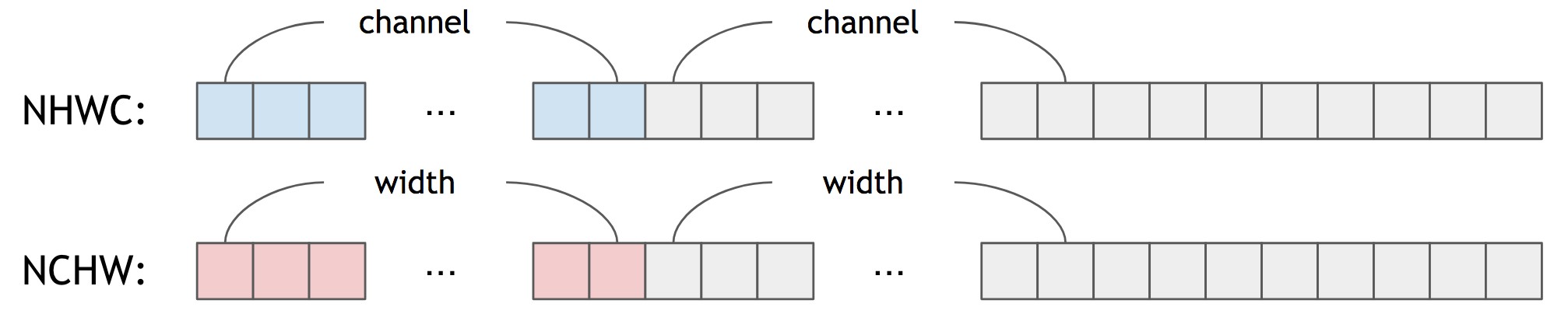
Figure 8. NHWC vs NCHW

换句话说，对于 NHWC，tensor 的临近元素保存的是 channel-wise 信息，而不是 spatial-wise. 对于任何的 channel size，优化代码都并不简单，除非在 softmax 层前后都添加 transpose 操作.
在该项目中，尝试假设 2-channel 输出，实现 softmax 层.

第三种，采用预计算的查询表(pre-calculated lookup table) 实现 softmax 层. 由于使用了 8-bit 量化和 2-class 输出(前景和背景)，因此仅有 65536(=256x256) 个量化的输入值的不同组合，其可以保存在查询表中：

for (int fg = 0; fg < 256; fg++) {
  for (int bg = 0; bg < 256; bg++) {
    // Dequantize
    float fg_real = input->params.scale * (fg - input->params.zero_point);
    float bg_real = input->params.scale * (bg - input->params.zero_point);

    // Pre-calculating Softmax Values
    ...

    // Quantize
    precalculated_softmaxx = static_cast<uint8_t>(clamped);
  }
}

<h2>总结</h2>

主要介绍了在移动设备上肖像分割中遇到的挑战和解决技巧.
主要关注于保持高分割精度，支持在如 Galaxy J7 等的旧移动设备上运行.

<h2>参考文献</h2>

[1] Rethinking Atrous Convolution for Semantic Image Segmentation
[2] Rethinking the Inception Architecture for Computer Vision
[3] MobileNets: Efficient Convolutional Neural Networks for Mobile Vision Applications
[4] MobileNetV2: Inverted Residuals and Linear Bottlenecks
[5] Quantization and Training of Neural Networks for Efficient Integer-Arithmetic-Only Inference