作者:天山老霸王
灰度共生矩阵法(GLCM, Gray-level co-occurrence matrix),就是通过计算灰度图像得到它的共生矩阵,然后透过计算该共生矩阵得到矩阵的部分特征值,来分别代表图像的某些纹理特征(纹理的定义仍是难点)。灰度共生矩阵能反映图像灰度关于方向、相邻间隔、变化幅度等综合信息,它是分析图像的局部模式和它们排列规则的基础。
Python 实现
1. fast_glcm.py
fast_glcm.py
#!--*--coding: utf-8--*--

import numpy as np
import cv2


def fast_glcm(img, vmin=0, vmax=255, nbit=8, kernel_size=5):
    mi, ma = vmin, vmax
    ks = kernel_size
    h,w = img.shape

    # digitize
    bins = np.linspace(mi, ma+1, nbit+1)
    gl1 = np.digitize(img, bins) - 1
    gl2 = np.append(gl1[:,1:], gl1[:,-1:], axis=1)

    # make glcm
    glcm = np.zeros((nbit, nbit, h, w), dtype=np.uint8)
    for i in range(nbit):
        for j in range(nbit):
            mask = ((gl1==i) & (gl2==j))
            glcm[i,j, mask] = 1

    kernel = np.ones((ks, ks), dtype=np.uint8)
    for i in range(nbit):
        for j in range(nbit):
            glcm[i,j] = cv2.filter2D(glcm[i,j], -1, kernel)

    glcm = glcm.astype(np.float32)
    return glcm


def fast_glcm_mean(img, vmin=0, vmax=255, nbit=8, ks=5):
    '''
    calc glcm mean
    '''
    h,w = img.shape
    glcm = fast_glcm(img, vmin, vmax, nbit, ks)
    mean = np.zeros((h,w), dtype=np.float32)
    for i in range(nbit):
        for j in range(nbit):
            mean += glcm[i,j] * i / (nbit)**2

    return mean


def fast_glcm_std(img, vmin=0, vmax=255, nbit=8, ks=5):
    '''
    calc glcm std
    '''
    h,w = img.shape
    glcm = fast_glcm(img, vmin, vmax, nbit, ks)
    mean = np.zeros((h,w), dtype=np.float32)
    for i in range(nbit):
        for j in range(nbit):
            mean += glcm[i,j] * i / (nbit)**2

    std2 = np.zeros((h,w), dtype=np.float32)
    for i in range(nbit):
        for j in range(nbit):
            std2 += (glcm[i,j] * i - mean)**2

    std = np.sqrt(std2)
    return std


def fast_glcm_contrast(img, vmin=0, vmax=255, nbit=8, ks=5):
    '''
    calc glcm contrast
    '''
    h,w = img.shape
    glcm = fast_glcm(img, vmin, vmax, nbit, ks)
    cont = np.zeros((h,w), dtype=np.float32)
    for i in range(nbit):
        for j in range(nbit):
            cont += glcm[i,j] * (i-j)**2

    return cont


def fast_glcm_dissimilarity(img, vmin=0, vmax=255, nbit=8, ks=5):
    '''
    calc glcm dissimilarity
    '''
    h,w = img.shape
    glcm = fast_glcm(img, vmin, vmax, nbit, ks)
    diss = np.zeros((h,w), dtype=np.float32)
    for i in range(nbit):
        for j in range(nbit):
            diss += glcm[i,j] * np.abs(i-j)

    return diss


def fast_glcm_homogeneity(img, vmin=0, vmax=255, nbit=8, ks=5):
    '''
    calc glcm homogeneity
    '''
    h,w = img.shape
    glcm = fast_glcm(img, vmin, vmax, nbit, ks)
    homo = np.zeros((h,w), dtype=np.float32)
    for i in range(nbit):
        for j in range(nbit):
            homo += glcm[i,j] / (1.+(i-j)**2)

    return homo


def fast_glcm_ASM(img, vmin=0, vmax=255, nbit=8, ks=5):
    '''
    calc glcm asm, energy
    '''
    h,w = img.shape
    glcm = fast_glcm(img, vmin, vmax, nbit, ks)
    asm = np.zeros((h,w), dtype=np.float32)
    for i in range(nbit):
        for j in range(nbit):
            asm  += glcm[i,j]**2

    ene = np.sqrt(asm)
    return asm, ene


def fast_glcm_max(img, vmin=0, vmax=255, nbit=8, ks=5):
    '''
    calc glcm max
    '''
    glcm = fast_glcm(img, vmin, vmax, nbit, ks)
    max_  = np.max(glcm, axis=(0,1))
    return max_


def fast_glcm_entropy(img, vmin=0, vmax=255, nbit=8, ks=5):
    '''
    calc glcm entropy
    '''
    glcm = fast_glcm(img, vmin, vmax, nbit, ks)
    pnorm = glcm / np.sum(glcm, axis=(0,1)) + 1./ks**2
    ent  = np.sum(-pnorm * np.log(pnorm), axis=(0,1))
    return ent


if __name__ == '__main__':

    from skimage import data

    img = data.camera()
    h,w = img.shape

    img[:,:w//2] = img[:,:w//2]//2+127

    nbit = 8
    ks = 5
    mi, ma = 0, 255
    glcm_mean = fast_glcm_mean(img, mi, ma, nbit, ks)
2. glcm example
示例如,
#!--*--coding: utf-8--*--
import numpy as np
from skimage import data
from matplotlib import pyplot as plt
import fast_glcm

if __name__ == '__main__':
    img = data.camera()
    h,w = img.shape
    glcm_mean = fast_glcm.fast_glcm_mean(img)

    plt.imshow(glcm_mean)
    plt.tight_layout()
    plt.show()
3. plot example
#!--*--coding: utf-8--*--

import numpy as np
from skimage import data
from matplotlib import pyplot as plt
import fast_glcm
from PIL import Image

def main():
    pass


if __name__ == '__main__':
    img_file = "test.jpg"
    img=np.array(Image.open(img_file).convert('L'))
    h,w = img.shape

    mean = fast_glcm.fast_glcm_mean(img)
    std = fast_glcm.fast_glcm_std(img)
    cont = fast_glcm.fast_glcm_contrast(img)
    diss = fast_glcm.fast_glcm_dissimilarity(img)
    homo = fast_glcm.fast_glcm_homogeneity(img)
    asm, ene = fast_glcm.fast_glcm_ASM(img)
    ma = fast_glcm.fast_glcm_max(img)
    ent = fast_glcm.fast_glcm_entropy(img)

    plt.figure(figsize=(10,4.5))
    fs = 15
    plt.subplot(2,5,1)
    plt.tick_params(labelbottom=False, labelleft=False)
    plt.imshow(img)
    plt.title('original', fontsize=fs)

    plt.subplot(2,5,2)
    plt.tick_params(labelbottom=False, labelleft=False)
    plt.imshow(mean)
    plt.title('mean', fontsize=fs)

    plt.subplot(2,5,3)
    plt.tick_params(labelbottom=False, labelleft=False)
    plt.imshow(std)
    plt.title('std', fontsize=fs)

    plt.subplot(2,5,4)
    plt.tick_params(labelbottom=False, labelleft=False)
    plt.imshow(cont)
    plt.title('contrast', fontsize=fs)

    plt.subplot(2,5,5)
    plt.tick_params(labelbottom=False, labelleft=False)
    plt.imshow(diss)
    plt.title('dissimilarity', fontsize=fs)

    plt.subplot(2,5,6)
    plt.tick_params(labelbottom=False, labelleft=False)
    plt.imshow(homo)
    plt.title('homogeneity', fontsize=fs)

    plt.subplot(2,5,7)
    plt.tick_params(labelbottom=False, labelleft=False)
    plt.imshow(asm)
    plt.title('ASM', fontsize=fs)

    plt.subplot(2,5,8)
    plt.tick_params(labelbottom=False, labelleft=False)
    plt.imshow(ene)
    plt.title('energy', fontsize=fs)

    plt.subplot(2,5,9)
    plt.tick_params(labelbottom=False, labelleft=False)
    plt.imshow(ma)
    plt.title('max', fontsize=fs)

    plt.subplot(2,5,10)
    plt.tick_params(labelbottom=False, labelleft=False)
    plt.imshow(ent)
    plt.title('entropy', fontsize=fs)

    plt.tight_layout(pad=0.5)
    plt.savefig('output.jpg')
    plt.show()
如,原图:

GLCM 结果图:
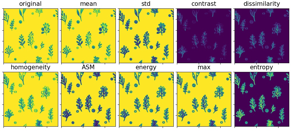
4. 结果含义
[1] - 均值(Mean)
[2] - 标准差(Std)
[3] - 对比度(Contrast)
对比度反应了图像的清晰度和纹理的沟纹深浅。度量矩阵的值是如何分布和图像中局部变化的多少,反应了图像的清晰度和纹理的沟纹深浅。纹理的沟纹越深,反差越大,效果清晰;反之,对比值小,则沟纹浅,效果模糊。
反应某像素值及其领域像素值亮度的对比情况,图像亮度值变化快,换句话说纹理较深,它的对比度就越大,也就是它的纹理越清晰。
[4] - 相异性(Dissimilarity)
计算对比度时,权重随矩阵元素与对角线的距离以指数方式增长,如果改为线性增长,则得到相异性。
[5] - 同质性/逆差距(Homogeneity)
测量图像的局部均匀性,非均匀图像的值较低,均匀图像的值较高。与对比度或相异性相反,同质性的权重随着元素值与对角线的距离而减小,其减小方式是指数形式的。
[6] - 角二阶矩 / 能量( ASM)
灰度共生矩阵( grey level co-occurrence matrix,GLCM)用来描述图像灰度分布的均匀程度和纹理的粗细程度。
如果 GLCM 的所有值都非常接近,则 ASM 值较小; 如果矩阵元素取值差别较大,则 ASM 值较大。当 ASM 值较大时,纹理粗,能量大; 反之,当 ASM 值小时,纹理细,能量小。
$$ ASM = \sum_i \sum_j P(i, j)^2 $$
[7] - 能量(Energy)
是灰度共生矩阵各元素值的平方和,是对图像纹理的灰度变化稳定程度的度量,反应了图像灰度分布均匀程度和纹理粗细度。能量值大表明当前纹理是一种规则变化较为稳定的纹理。更高的值==纹理均匀性。
[8] - 熵(Entropy)
测量图像纹理的随机性(强度分布)。熵是图像包含信息量的随机性度量,表现了图像的复杂程度。当共生矩阵中所有值均相等或者像素值表现出最大的随机性时,熵最大;因此熵值表明了图像灰度分布的复杂程度,熵值越大,图像越复杂。
表示矩阵中元素的分散程度,也表示图像纹理的复杂程度。
[9] - 最大概率(Maximum probability)
表示图像中出现次数最多的纹理特征。
1 条评论
博主您好,我是一个小白,我想请教一下代码问题:就是您在上面写的代码如下,下面这段代码中
gl2 = np.append(gl1[:,1:], gl1[:,-1:], axis=1)
这行代码的意义是什么我不是很理解,还有下面一行嵌套循环的意思是什么?能帮我解答一下吗?十分感谢!