原文:EINSUM IS ALL YOU NEED - EINSTEIN SUMMATION IN DEEP LEARNING - 2018.05.02
译文:einsum满足你一切需要:深度学习中的爱因斯坦求和约定
作者:TIM ROCKTASCHEL
节选,学习.
1. einsum 标记法
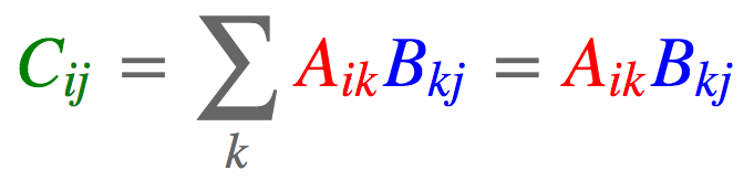
1.1. 矩阵相乘
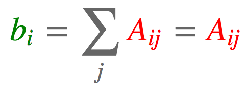
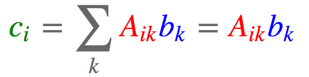
比如,两个矩阵相乘,$A \in R^{I \times K}$ 和 $B \in R^{K \times J}$ ;再计算每列的和,最终得到矩阵 $c \in R^J$,其可以表达为:
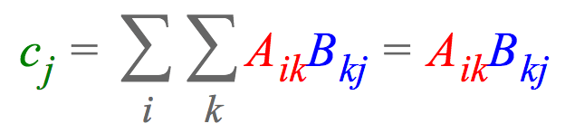
其中,表达式说明了每个元素 $c_i$ 的计算过程. 列向量 $A_{i:}$ 乘以行向量 $B_{:j}$,再求和.
einsum 标记法中,隐式地省略了求和符号,而是累加重复的下标(如,$k$) 和输出中未标出的下标(如 $i$).
1.2. 向量点积
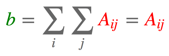
比如,两个向量 $a, b \in R^{J}$ 的点积,可以表达为:

1.3. 高阶张量变换
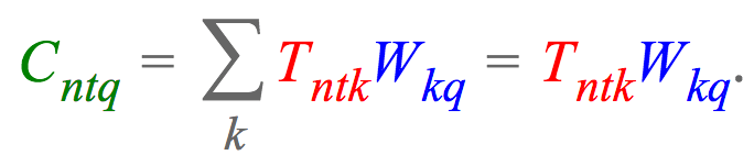
比如,深度学习常见的一种高阶张量(higher-order tensor),其包含一个 batch 中有 N 个训练样本,每个样本是一个长度为 T 的 K 维词向量序列,期望将词向量投影到一个不同的维度 Q.
记,张量为 $T \in R^{N \times T \times K}$,投影矩阵记为 $W \in R^{K \times Q}$,则,einsum 表达式为:
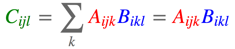
1.4. 四阶张量变换
比如,对于四阶张量 $T \in R^{N \times T \times K \times M}$,期望使用上述的投影矩阵 W 将第三维投影到 Q 维,并累加到第二维,再对结果中的第一维和最后一维进行转置,最终得到张量 $C \in R^{M \times Q \times N}$. einsum 表达式为:

注,这里是通过交换下标 n 和 m ($C_{mqn}$ 而不是 $C_{nqm}$),转置了张量结果.
2. Numpy/PyTorch/TensorFlow 中 einsum 标记法
NumPy - einsum 符号标记函数 - AIUAI
Numpy - np.einsum
PyTorch - torch.einsum
TensorFlow - tf.einsum
表示形式均为:
einsum(equation, operands)
#equation - einsum 约定字符串
#operands - 张量序列如,1.1.矩阵相乘,$c_j = \sum _i \sum_k A_{ik} B_{kj}$,其表示形式如:
equation = 'ik,kj -> j'Numpy/PyTorch/TensorFlow 支持 einsum 的好处在于,可以应用于神经网络架构中的任意计算图,且可以反向传播.
典型 einsum 调用形式如:

其中,方框是占位符,表示张量维度. 根据该式,可以推断,arg1 和 arg3 是矩阵,arg2 是三阶张量,einsum 计算结果 result 是矩阵.
注意,einsum 处理的是可变数量的输入.
以下依PyTorch为例示例介绍.
2.1. 矩阵转置

import torch

a = torch.arange(6).reshape(2, 3)
#tensor([[0, 1, 2],
#        [3, 4, 5]])
b = torch.einsum('ij->ji', [a])
#tensor([[0, 3],
#        [1, 4],
#        [2, 5]])
2.2. 求和
import torch

a = torch.arange(6).reshape(2, 3)
b = torch.einsum('ij->', [a])
#tensor(15)
2.3. 列求和
import torch

a = torch.arange(6).reshape(2, 3)
b = torch.einsum('ij->j', [a])
#tensor([3, 5, 7])
2.4. 行求和
import torch

a = torch.arange(6).reshape(2, 3)
b = torch.einsum('ij->i', [a])
#tensor([ 3, 12])
2.5. 矩阵-向量相乘
import torch

a = torch.arange(6).reshape(2, 3)
b = torch.arange(3)
#tensor([0, 1, 2])
c = torch.einsum('ik,k->i', [a, b])
#tensor([ 5, 14])
2.6. 矩阵-矩阵相乘
import torch

a = torch.arange(6).reshape(2, 3)
b = torch.arange(15).reshape(3, 5)
#tensor([[ 0,  1,  2,  3,  4],
#        [ 5,  6,  7,  8,  9],
#        [10, 11, 12, 13, 14]])
c = torch.einsum('ik,kj->ij', [a, b])
#tensor([[ 25,  28,  31,  34,  37],
#        [ 70,  82,  94, 106, 118]])
2.7. 向量点积

import torch

a = torch.arange(3)
#tensor([0, 1, 2])
b = torch.arange(3,6)
#tensor([3, 4, 5])
c = torch.einsum('i,i->', [a, b])
#tensor(14)
2.8. 矩阵点积

import torch

a = torch.arange(6).reshape(2, 3)
#tensor([[0, 1, 2],
#        [3, 4, 5]])
b = torch.arange(6,12).reshape(2, 3)
#tensor([[ 6,  7,  8],
#        [ 9, 10, 11]])
c = torch.einsum('ij,ij->', [a, b])
#tensor(145)
2.9. 哈达玛积(hadamard product)
逐元素相乘

import torch

a = torch.arange(6).reshape(2, 3)
b = torch.arange(6,12).reshape(2, 3)
c = torch.einsum('ij,ij->ij', [a, b])
#tensor([[ 0,  7, 16],
#        [27, 40, 55]])
2.10. 外积

import torch

a = torch.arange(3)
#tensor([0, 1, 2])
b = torch.arange(3,7)
#tensor([3, 4, 5, 6])
c = torch.einsum('i,j->ij', [a, b])
#tensor([[ 0,  0,  0,  0],
#        [ 3,  4,  5,  6],
#        [ 6,  8, 10, 12]])
2.11. batch矩阵相乘
import torch

a = torch.randn(3,2,5)
#tensor([[[ 0.5950, -0.5277, -2.9840,  1.2765,  0.7984],
#         [-0.6398, -1.2514,  0.7914, -0.0121, -1.7285]],
#
#        [[ 0.2307, -1.4304,  1.4129,  1.5815,  0.9152],
#         [ 1.1122, -0.8018, -0.7850, -0.3227, -1.3101]],
#
#        [[ 0.4733,  0.0346,  0.5624, -0.4903, -0.2846],
#         [ 0.5879, -2.5767, -0.9281, -0.2841, -0.7726]]])
b = torch.randn(3,5,3)
#tensor([[[ 0.2185,  0.9919,  0.8251],
#         [ 1.2944,  0.1446,  1.6375],
#         [-0.3014,  0.7044, -0.6302],
#         [ 0.8771,  0.5083,  0.2780],
#         [-0.3134, -0.6291, -0.5817]],
#
#        [[ 0.0386,  0.6317, -0.7736],
#         [-0.2040, -0.0580,  0.3656],
#         [ 0.3501,  0.1585,  3.0762],
#         [-0.3240,  1.7353, -0.6806],
#         [-0.2196, -3.0822, -0.3082]],
#
#        [[ 0.4036,  0.3139, -0.5903],
#         [-0.3245,  1.5031,  0.4882],
#         [-0.5755, -0.4293,  1.4693],
#         [-0.4305,  0.5471, -1.6474],
#         [-0.1197,  0.1413,  1.1977]]])
c = torch.einsum('ijk,ikl->ijl', [a, b]) #torch.Size([3, 2, 3])
#tensor([[[ 1.2156, -1.4416,  1.3977],
#         [-1.4670,  0.8232, -2.0737]],
#
#        [[ 0.0818,  0.3761,  2.2866],
#         [ 0.3240,  4.1028, -2.9448]],
#
#        [[ 0.1012, -0.3493,  1.0307],
#         [ 1.8223, -3.5545, -3.4262]]])
2.12. 张量缩约(tensor contraction)
batch 矩阵相乘是 tensor contraction 特殊情况.
比如两个张量,一个 n 阶张量 $A \in R^{I_1 \times \cdot \times I_n }$,一个 m 阶张量 $B \in R^{J_1 \times \cdot \times J_m}$.
举例来说,假设 n=4, m=5,且假定 $I_2 = J_3$ 且 $I_3 = J_5$.
可以将这两个张量在这两个维度上相乘(A 张量的第 2、3 维度,B 张量的 3、5 维度),最终得到一个新张量 $C \in R^{I1 \times I4 \times J1 \times J2 \times J4}$,如下式,

import torch

a = torch.randn(2,3,5,7)
b = torch.randn(11,13,3,17,5)

c = torch.einsum('pqrs,tuqvr->pstuv', [a, b]).shape
#torch.Size([2, 7, 11, 13, 17])
2.13. 双线性变换
einsum 可用于超过两个张量的计算,如,双线性变换,

import torch

a = torch.randn(2,3)
b = torch.randn(5,3,7)
c = torch.randn(2,7)
#
d = torch.einsum('ik,jkl,il->ij', [a, b, c])
#tensor([[ 0.8701, -0.7686,  3.2942,  5.8559, -2.3225],
#        [ 0.9466,  0.5451,  0.4778, -0.4806, -1.8109]])
3. 示例
3.1. TreeQN
比如,TreeQN 中等式 6 的实现. 给定网络层 $l$ 的低维状态表示 $z_l$ 以及每个激活函数 $a$ 的转换函数 $W^a$,期望计算采用了残差链接后的所有下一层状态 $z_{l+1}^a$:
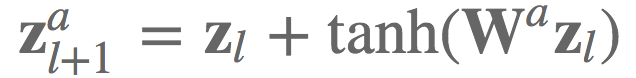
实际场景中,想要高效的地酸 batch 为 B 的 K 维状态表示 $Z \in R^{B \times K}$,并同时计算所有的转换函数(即,所有激活函数A),可以将这些转换函数表示为一个张量 $W \in R^{A \times K \times K}$,并使用 einsum 标记法高效的计算下一层状态表示.
import torch.nn.functional as F

def random_tensors(shape, num=1, requires_grad=False):
  tensors = [torch.randn(shape, requires_grad=requires_grad) for i in range(0, num)]
  return tensors[0] if num == 1 else tensors

#参数
#-- [num_actions x hidden_dimension]
#-- [激活函数数 x 隐藏层维度]
b = random_tensors([5, 3], requires_grad=True)
#-- [num_actions x hidden_dimension x hidden_dimension]
#-- [激活函数数 x 隐藏层维度 x 隐藏层维度]
W = random_tensors([5, 3, 3], requires_grad=True)

def transition(zl):
    #-- [batch大小 x 激活函数数 x 隐藏层维度]
    #-- [batch_size x num_actions x hidden_dimension]
    return zl.unsqueeze(1) + F.tanh(torch.einsum("bk,aki->bai", [zl, W]) + b)

#随机生成输入
#-- [batch大小 x 隐藏层维度]
zl = random_tensors([2, 3])

#
out = transition(zl)
3.2. Attention
论文 Reasoning about Entailment with Neural Attention - ICLR2016 中注意力机制的等式 11- 13:
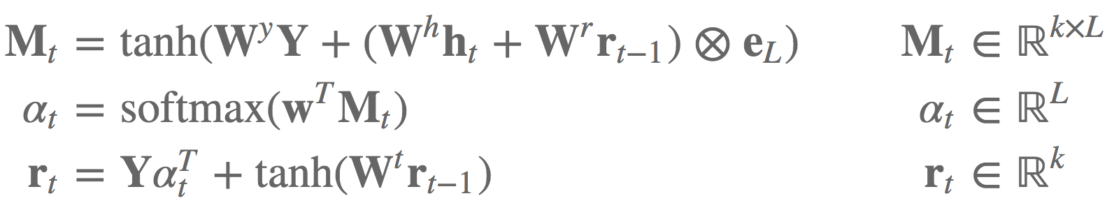
einsum 标记法实现如:
#参数
#-- [隐藏层维度]
bM, br, w = random_tensors([7], num=3, requires_grad=True)
#-- [隐藏层维度 x 隐藏层维度]
WY, Wh, Wr, Wt = random_tensors([7, 7], num=4, requires_grad=True)

#单次注意力机制
def attention(Y, ht, rt1):
    #-- [batch大小 x 隐藏层维度]
    tmp = torch.einsum("ik,kl->il", [ht, Wh]) + torch.einsum("ik,kl->il", [rt1, Wr])
    Mt = F.tanh(torch.einsum("ijk,kl->ijl", [Y, WY]) + tmp.unsqueeze(1).expand_as(Y) + bM)
    #-- [batch大小 x 序列长度]
    at = F.softmax(torch.einsum("ijk,k->ij", [Mt, w]))
    #-- [batch大小 x 隐藏层维度]
    rt = torch.einsum("ijk,ij->ik", [Y, at]) + F.tanh(torch.einsum("ij,jk->ik", [rt1, Wt]) + br)
    #-- [batch大小 x 隐藏层维度], [batch大小 x 序列维度]
    return rt, at

#随机生成输入
#-- [batch大小 x 序列长度 x 隐藏层维度]
Y = random_tensors([3, 5, 7])
# -- [batch大小 x 隐藏层维度]
ht, rt1 = random_tensors([3, 7], num=2)

rt, at = attention(Y, ht, rt1)
print(at) #打印注意力权重
3.3. Moco
MoCo: Momentum Contrast for Unsupervised Visual Representation Learning 中也有相应的实现.
Pytorch 伪代码(部分):
q = f_q.forward(x_q) # queries: NxC
k = f_k.forward(x_k) # keys: NxC
k = k.detach() # no gradient to keys
# positive logits: Nx1
l_pos = bmm(q.view(N,1,C), k.view(N,C,1))
# negative logits: NxK
l_neg = mm(q.view(N,C), queue.view(C,K))
# logits: Nx(1+K)
logits = cat([l_pos, l_neg], dim=1)
Pytorch 中的实现 - moco/builder.py:
# compute logits
# Einstein sum is more intuitive
# positive logits: Nx1
l_pos = torch.einsum('nc,nc->n', [q, k]).unsqueeze(-1)
# negative logits: NxK
l_neg = torch.einsum('nc,ck->nk', [q, self.queue.clone().detach()])

# logits: Nx(1+K)
logits = torch.cat([l_pos, l_neg], dim=1)
2 条评论
博主您好,想问一下moco的这个算法是啥意思torch.einsum('nc,nc->n', [q, k]),我一直不理解,上面我也没有找到响应的例子
参考这个,
输入shape 是 nc 与 nc; 输出shape 是 nx1.