1. KNN
1.1. KNN sklearn
import numpy as np
from sklearn.neighbors import NearestNeighbors

features = np.array() #NxC
n_neighbors = 100 #KNN 中 k 的个数
nbrs = NearestNeighbors(n_neighbors=n_neighbors, metric='euclidean').fit(features)
knn_distances, knn_neighbor_indices = nbrs.kneighbors(features)
1.2. KNN 存在的问题
虽然 KNN 能够有效的找到相似样本,但其需要进行大量的成对距离计算. 如果数据集包含 1000 个样本,对于一个新样本,查询其 K=3 个最近邻,则,KNN 算法需要进行 1000 次距离计算. 好像还不太坏. 但,设想下,对于一个 C2C 的市场,数据库中包含百万级商品,每天更新成千上万的的新产品. KNN 的计算量就太大且费时了.
为了减少计算量,避免暴力的距离计算,而使用一种更复杂的算法,即:ANN(Approximate Nearest Neighbors).
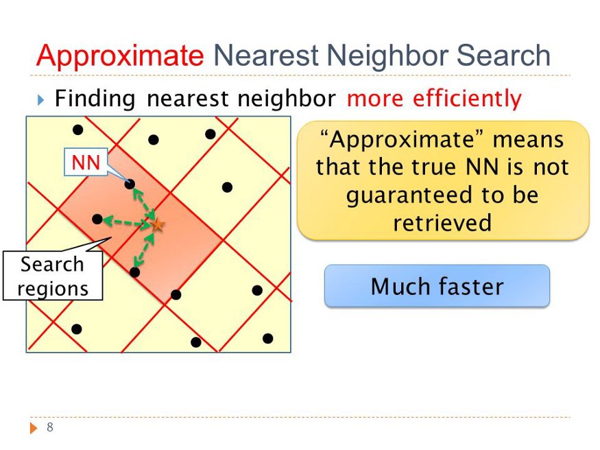
2. ANN
ANN 是一类算法,其允许在最近邻搜索时有少量的误差. 不过,在真实的 C2C 业务场景中,真正的邻近样本数是远超过要搜索的 K 个最近邻样本. ANN 算法仅需 KNN 暴力匹配的部分时间,即可取得相当的精度.
几种 ANN 算法如,
[1] - HNSW(Hierarchical Navigable Small World graphs)
[2] - Faiss - Facebook
[3] - ANNOY - Spotify
[4] - ScaNN - Google
2.1. HNSW
安装:
pip install hnswlib
#或:
git clone https://github.com/nmslib/hnswlib.git
cd hnswlib
pip install .
示例如:
import hnswlib
import numpy as np

#创建 HNSW 索引
def fit_hnsw_index(features, ef=100, M=16, save_index_file=False):
    # HNSW图构建的辅助函数
    # features: 特征列表,每一行是一个特征
    # ef 和 M: HNSW算法的参数

    num_elements = len(features)
    labels_index = np.arange(num_elements)
    EMBEDDING_SIZE = len(features[0])

    #Declaring index,声明索引类型,如:l2, cosine or ip
    p = hnswlib.Index(space='l2', dim=EMBEDDING_SIZE)

    #Initing index - the maximum number of elements should be known
    #初始化索引,元素的最大数需要是已知的
    p.init_index(max_elements=num_elements, ef_construction=ef, M=M)

    #Element insertion,插入数据
    int_labels = p.add_items(features, labels_index)

    # Controlling the recall by setting ef
    # ef should always be > k
    # 设置ef控制召回率
    p.set_ef(ef)

    #是否将索引图保存到本地文件
    if save_index_file:
         p.save_index(save_index_file)

    return p

#查询K近邻
ann_neighbor_indices, ann_distances = p.knn_query(features, k)
HNSW 支持的距离计算方式:
| Distance | parameter | Equation |
|---|---|---|
| Squared L2 | 'l2' | d = sum((Ai-Bi)^2) |
| Inner product | 'ip' | d = 1.0 - sum(Ai * Bi) |
| Cosine similarity | 'cosine' | d = 1.0 - sum(Ai * Bi) / sqrt(sum(Ai * Ai) * sum(Bi * Bi)) |
2.2. Faiss
安装:
pip install faiss
#https://github.com/facebookresearch/faiss
示例如,
import numpy as np
import faiss


class FaissKNeighbors:
    def __init__(self, k=5):
        self.index = None #索引类
        self.y = None
        self.k = k

    def fit(self, X, y):
        self.index = faiss.IndexFlatL2(X.shape[1]) #欧式距离,L2Norm,非常类似于scikit-learn KNeighborsClassifier
        self.index.add(X.astype(np.float32)) #索引的数据类型是 Numpy float32.
        self.y = y

    def predict(self, X):
        #返回KNN的距离和索引.
        distances, indices = self.index.search(X.astype(np.float32), k=self.k)
        #indices 是 2D 矩阵形式
        votes = self.y[indices]
        #X中最多的数,即预测的标签. 逐行进行.
        predictions = np.array([np.argmax(np.bincount(x)) for x in votes])
        return predictions
2.3. Annoy
安装:
pip install annoy
#https://github.com/spotify/annoy
示例如:
from annoy import AnnoyIndex

f = 3 #待构建索引的向量长度
metric = 'angular' #距离度量,可选:"angular", "euclidean", "manhattan", "hamming", or "dot".
a = AnnoyIndex(f, metric)
a.add_item(0, [1, 0, 0]) #添加样本
a.add_item(1, [0, 1, 0])
a.add_item(2, [0, 0, 1])
a.build(-1)
#a.build(n_trees, n_jobs=-1),构建 n_trees 树的随机森林
#  n_jobs 指定构建树时的线程数,n_jobs=-1 表示所有可用的 CPU 核.
#a.save(fn, prefault=False) #保存索引到本地.
#a.load(fn, prefault=False) #从本地加载索引.


a.get_nns_by_item(0, 100) #查询 100 个最近邻样本
a.get_nns_by_vector([1.0, 0.5, 0.5], 100) #向量查询
a.get_item_vector(i) #返回先前添加的样本i的向量
a.get_distance(i, j) #计算i和j之间的距离
a.get_n_items() #返回索引中样本(items)数
a.get_n_trees() #返回索引中数(trees)数
annoy/precision_test.py
from __future__ import print_function
import random, time
from annoy import AnnoyIndex

try:
    xrange
except NameError:
    # Python 3 compat
    xrange = range

n, f = 100000, 40
t = AnnoyIndex(f, 'angular') #索引
#添加样本
for i in xrange(n):
    v = []
    for z in xrange(f):
        v.append(random.gauss(0, 1))
    t.add_item(i, v)
#构建索引
t.build(2 * f)
#保存到本地
t.save('test.tree')

limits = [10, 100, 1000, 10000]
k = 10
prec_sum = {}
prec_n = 1000
time_sum = {}
for i in xrange(prec_n):
    j = random.randrange(0, n)
    #计算最近邻
    closest = set(t.get_nns_by_item(j, k, n))
    for limit in limits:
        t0 = time.time()
        toplist = t.get_nns_by_item(j, k, limit)
        T = time.time() - t0

        found = len(closest.intersection(toplist))
        hitrate = 1.0 * found / k
        prec_sum[limit] = prec_sum.get(limit, 0.0) + hitrate
        time_sum[limit] = time_sum.get(limit, 0.0) + T

for limit in limits:
    print('limit: %-9d precision: %6.2f%% avg time: %.6fs'
          % (limit, 100.0 * prec_sum[limit] / (i + 1),
             time_sum[limit] / (i + 1)))
2.4. Scann
安装:
pip install scann
#https://github.com/google-research/google-research/tree/master/scann
Scann 向量搜索包括三个方面:
[1] - Partition(可选):训练时将数据集分区,查询时选择top个分区到 score 阶段;
[2] - Score: 计算查询样本与数据集样本的距离(如果没有开启 Partition);或着,查询样本与分区样本之间的距离;计算的距离不一定是精确的.
[3] - Rescore(可选):从 Score 的结果中选择最佳的 k 个距离,重新更精确的计算距离.
Scann 经验规则(rules-of-thumb):
[1] - 对于数据量少于 20K 的小数据集,采用暴力法(brute-force).
[2] - 对于数据量小于 100K 的数据集,采用先 score with AH,再 rescore.
[3] - 对于数据量大于 100K 的数据集,采用先 partition,再 score with AH,再 rescore.
[4] - 当采用 score with AH 时,dimensions_per_block 应该设置为 2.
[5] - 当采用 partition 时,num_leaves 应该粗略的设置为数据样本数的平方根.
示例如:
import numpy as np

import scann

normalized_dataset = '' #NxC
queries = '' #NxC

#创建 ScaNN 搜索器
#配置 ScaNN 树
# use scann.scann_ops.build() to instead create a TensorFlow-compatible searcher
#这里,搜索 2000 个叶节点中的 top100,再精确计算 top100 的内积,以返回最终的 top10结果.
searcher = scann.scann_ops_pybind.builder(normalized_dataset, 10, "dot_product").tree(
    num_leaves=2000, num_leaves_to_search=100, training_sample_size=250000).score_ah(
    2, anisotropic_quantization_threshold=0.2).reorder(100).build()

#
def compute_recall(neighbors, true_neighbors):
    total = 0
    for gt_row, row in zip(true_neighbors, neighbors):
        total += np.intersect1d(gt_row, row).shape[0]
    return total / true_neighbors.size

#查询top10
start = time.time()
neighbors, distances = searcher.search_batched(queries)
end = time.time()

print("Recall:", compute_recall(neighbors, true_neighbors)
print("Time:", end - start)

#
#增加叶节点数,以提升 recall,同时计算速度
start = time.time()
neighbors, distances = searcher.search_batched(queries, leaves_to_search=150)
end = time.time()

print("Recall:", compute_recall(neighbors, glove_h5py['neighbors'][:, :10]))
print("Time:", end - start)

#增加重排序(top AH 候选结果的精确评分)
start = time.time()
neighbors, distances = searcher.search_batched(queries, leaves_to_search=150, pre_reorder_num_neighbors=250)
end = time.time()

print("Recall:", compute_recall(neighbors, glove_h5py['neighbors'][:, :10]))
print("Time:", end - start)

#
neighbors, distances = searcher.search_batched(queries, final_num_neighbors=20)
print(neighbors.shape, distances.shape)

#
#单条查询
start = time.time()
neighbors, distances = searcher.search(queries[0], final_num_neighbors=5)
end = time.time()

print(neighbors)
print(distances)
print("Latency (ms):", 1000*(end - start))
参考
[1] - Make kNN 300 times faster than Scikit-learn’s in 20 lines - 2020.09.12
[2] - Faiss indexes
[3] - https://github.com/piyushpathak03/Approximate-Nearest-Neighbors/blob/main/knn_is_dead.ipynb