原文 - 实战 | Elasticsearch自定义评分的N种方法 - 2020.03.11
相似性(similarity,scoring/ranking model)定义了文档匹配的分数.
相似性是每个字段的(per field),也就是说,通过 mapping,可以对每个字段定义不同的相似性.
1. ElasticSearch 相关性
结构化数据库如Mysql,只能查询结果与数据库中的row的是否匹配?回答往往是“是”、“否”.
如:
select title from hbinfos where title like ‘%发热%’。而全文搜索引擎Elasticsearch 中不仅需要找到匹配的文档,还需根据它们相关度的高低进行排序.
实现相关度排序的核心概念是评分.
_score就是Elasticsearch检索返回的评分,该得分衡量每个文档与查询的匹配程度.
 "hits" : [
      {
        "_index" : "kibana_sample_data_flights",
        "_type" : "_doc",
        "_id" : "FHLWlHABl_xiQyn7bHe2",
        "_score" : 3.4454226,
        }]
每个文档都有与之相关的评分,该得分由正浮点数表示. 文档分数越高,则文档越相关.
分数与查询匹配成正比. 查询中的每个子句都将有助于文档的得分.
2. ElasticSearch 相似性计算
ElasticSearch - simlilarity
Elasticsearch使用布尔模型查找匹配文档,并用一个名为实用评分函数的公式来计算相关度. 这个公式借鉴了词频/逆向文档频率和向量空间模型,同时也加入了一些现代的新特性,如协调因子(coordination factor),字段长度归一化(field length normalization),以及词或查询语句权重提升。
Elasticsearch 5 之前的版本,评分机制或者打分模型基于 TF-IDF 实现. 从Elasticsearch 5之后, 缺省的打分机制改成了Okapi BM25**。
BM25 的 BM 是缩写自 Best Match, 25 貌似是经过 25 次迭代调整之后得出的算法,它也是基于 TF/IDF 进化来的。
示例如,
PUT my-index-000001
{
  "mappings": {
    "properties": {
      "default_field": { #默认采用 BM25 相似性
        "type": "text"
      },
      "boolean_sim_field": {
        "type": "text",
        "similarity": "boolean"  #采用 boolean 相似性
      }
    }
  }
2.1. TF-IDF 和 BM25 相同点
TF-IDF 和 BM25 同样使用逆向文档频率来区分普通词(不重要)和非普通词(重要),同样认为:
[1] - 文档里的某个词出现次数越频繁,文档与这个词就越相关,得分越高。
[2] - 某个词在集合所有文档里出现的频率是多少?频次越高,权重 越低,得分越低 。某个词在集合中所有文档中越罕见,得分越高。
2.2. TF-IDF 和 BM25 不同点
BM25在传统TF-IDF的基础上增加了几个可调节的参数,使得它在应用上更佳灵活和强大,具有较高的实用性。
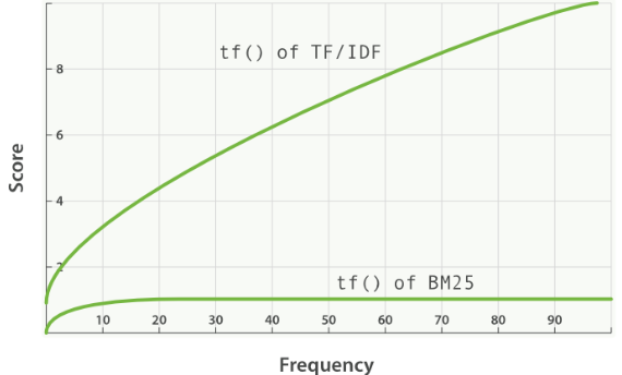
[1] - 传统的TF值理论上是可以无限大的。而BM25与之不同,它在TF计算方法中增加了一个常量k,用来限制TF值的增长极限。下面是两者的公式:
$$ \text{传统 TF_Score} = sqrt(tf) $$
$$ \text{BM25 TF_Score} = \frac{(k+1) * tf}{k + tf} $$
[2] - BM25还引入了平均文档长度的概念,单个文档长度对相关性的影响力与它和平均长度的比值有关系. BM25的TF公式里,除了常量k外,引入另外两个参数:L和b.
$$ \text{TF_Score} = \frac{(k+1) * tf}{k * (1.0 - b + b*L) + tf} $$
更多细节原理推荐:
https://blog.mimacom.com/elasticsearch-scoring-algorithm-changes/
3. ElasticSearch 相似性查询
ElasticSearch 布尔查询中,每个must,should和must_not元素称为查询子句.
[1] - 文档满足 must 或 should 的标准的程度有助于文档的相关性得分. 分数越高,文档就越符合搜索条件。
[2] - must_not子句中的条件被视为过滤器. 它会影响文档是否包含在结果中,但不会影响文档的评分方式. 在must_not里还可以显式指定任意过滤器,以基于结构化数据包括或排除文档.
[3] - filter:必须匹配,但它以不评分、过滤模式来进行. filter内部语句对评分没有贡献,只是根据过滤标准来排除或包含文档.
一句话概括:filter、must_not 不影响评分,其他影响评分.
4. ElasticSearch 自定义相似性
ElasticSearch - Similarity module
4.1. 配置相似性
大部分相似性计算,可以通过 index 配置来进行设定,如:
默认相似性:
PUT /index
{
  "settings": {
    "index": {
      "similarity": {
        "default": {
          "type": "boolean"
        }
      }
    }
  }
}
当创建索引(index)后,如果要更改默认相似性,则需要关闭原索引,并重新打开:
POST /index/_close?wait_for_active_shards=0

PUT /index/_settings
{
  "index": {
    "similarity": {
      "default": {
        "type": "boolean"
      }
    }
  }
}

POST /index/_open
DFR 相似性:
PUT /index
{
  "settings": {
    "index": {
      "similarity": {
        "my_similarity": {
          "type": "DFR",
          "basic_model": "g",
          "after_effect": "l",
          "normalization": "h2",
          "normalization.h2.c": "3.0"
        }
      }
    }
  }
}
该示例中,配置了 DFR 相似性,其可以在 mapping 中作为 my_similarity 进行使用,如:
PUT /index/_mapping
{
  "properties" : {
    "title" : { "type" : "text", "similarity" : "my_similarity" }
  }
}
4.2. 可用相似性
[1] - BM25 - Okapi_BM25
[2] - DFR - divergence from randomness framework
[3] - DFI - divergence from independence model
[4] - IB - Information based model
[5] - LMDirichlet - LM Dirichlet similarity
[6] - LMJelinekMercer - LM Jelinek Mercer similarity
4.3. 使用脚本定义相似性
ElasticSearch 支持通过脚本来定义相似性,例如,TF-IDF 脚本:
PUT /index
{
  "settings": {
    "number_of_shards": 1,
    "similarity": {
      "scripted_tfidf": {
        "type": "scripted",
        "script": {
          "source": "double tf = Math.sqrt(doc.freq); double idf = Math.log((field.docCount+1.0)/(term.docFreq+1.0)) + 1.0; double norm = 1/Math.sqrt(doc.length); return query.boost * tf * idf * norm;"
        }
      }
    }
  },
  "mappings": {
    "properties": {
      "field": {
        "type": "text",
        "similarity": "scripted_tfidf"
      }
    }
  }
}

PUT /index/_doc/1
{
  "field": "foo bar foo"
}

PUT /index/_doc/2
{
  "field": "bar baz"
}

POST /index/_refresh

GET /index/_search?explain=true
{
  "query": {
    "query_string": {
      "query": "foo^1.7",
      "default_field": "field"
    }
  }
}
其输出结果,如:
{
  "took": 12,
  "timed_out": false,
  "_shards": {
    "total": 1,
    "successful": 1,
    "skipped": 0,
    "failed": 0
  },
  "hits": {
    "total": {
        "value": 1,
        "relation": "eq"
    },
    "max_score": 1.9508477,
    "hits": [
      {
        "_shard": "[index][0]",
        "_node": "OzrdjxNtQGaqs4DmioFw9A",
        "_index": "index",
        "_type": "_doc",
        "_id": "1",
        "_score": 1.9508477,
        "_source": {
          "field": "foo bar foo"
        },
        "_explanation": {
          "value": 1.9508477,
          "description": "weight(field:foo in 0) [PerFieldSimilarity], result of:",
          "details": [
            {
              "value": 1.9508477,
              "description": "score from ScriptedSimilarity(weightScript=[null], script=[Script{type=inline, lang='painless', idOrCode='double tf = Math.sqrt(doc.freq); double idf = Math.log((field.docCount+1.0)/(term.docFreq+1.0)) + 1.0; double norm = 1/Math.sqrt(doc.length); return query.boost * tf * idf * norm;', options={}, params={}}]) computed from:",
              "details": [
                {
                  "value": 1.0,
                  "description": "weight",
                  "details": []
                },
                {
                  "value": 1.7,
                  "description": "query.boost",
                  "details": []
                },
                {
                  "value": 2,
                  "description": "field.docCount",
                  "details": []
                },
                {
                  "value": 4,
                  "description": "field.sumDocFreq",
                  "details": []
                },
                {
                  "value": 5,
                  "description": "field.sumTotalTermFreq",
                  "details": []
                },
                {
                  "value": 1,
                  "description": "term.docFreq",
                  "details": []
                },
                {
                  "value": 2,
                  "description": "term.totalTermFreq",
                  "details": []
                },
                {
                  "value": 2.0,
                  "description": "doc.freq",
                  "details": []
                },
                {
                  "value": 3,
                  "description": "doc.length",
                  "details": []
                }
              ]
            }
          ]
        }
      }
    ]
  }
}
一种更有效的实现,
PUT /index
{
  "settings": {
    "number_of_shards": 1,
    "similarity": {
      "scripted_tfidf": {
        "type": "scripted",
        "weight_script": {
          "source": "double idf = Math.log((field.docCount+1.0)/(term.docFreq+1.0)) + 1.0; return query.boost * idf;"
        },
        "script": {
          "source": "double tf = Math.sqrt(doc.freq); double norm = 1/Math.sqrt(doc.length); return weight * tf * norm;"
        }
      }
    }
  },
  "mappings": {
    "properties": {
      "field": {
        "type": "text",
        "similarity": "scripted_tfidf"
      }
    }
  }
}
5. ElasticSearch 相关性实战问题
实战 | Elasticsearch自定义评分的N种方法 - 2020.03.11
核心是通过修改评分修改文档相关性,在最前面返回用户最期望的结果.
5.1. Index Boost 索引层面修改相关性
[1] - 原理说明:
允许在跨多个索引搜索时为每个索引配置不同的级别
[2] - 适用场景:
索引级别调整评分。
[3] - 实战举例:
一批数据里,有不同的标签,数据结构一致,不同的标签存储到不同的索引(A、B、C),最后要严格按照标签来分类展示的话,用什么查询比较好?
要求:先展示A类,然后B类,然后C类
PUT index_a/_doc/1
{
  "subject": "subject 1"
}
PUT index_b/_doc/1
{
  "subject": "subject 1"
}
PUT index_c/_doc/1
{
  "subject": "subject 1"
}


GET index_*/_search
{
  "indices_boost": [
    {
      "index_a": 1.5
    },
    {
      "index_b": 1.2
    },
    {
      "index_c": 1
    }
  ],
  "query": {
    "term": {
      "subject.keyword": {
        "value": "subject 1"
      }
    }
  }
}
5.2. boosting 修改文档相关性
boosting分为两种类型:
5.2.1. 索引期间修改文档的相关性
PUT my_index
{
  "mappings": {
    "properties": {
      "title": {
        "type": "text",
        "boost": 2
      }
    }
  }
}索引期间修改相关性的弊端非常明显:修改boost值的唯一方式是重建索引,reindex数据,成本太高了.
5.2.2. 查询时修改文档的相关性
[1] - 原理说明
通过boosting修改文档相关性。
boost取值:0 - 1 之间的值,如:0.2,代表降低评分;
boost取值:> 1, 如:1.5,代表提升评分。
[2] - 适用场景
自定义修改满足某个查询条件的评分.
[3] - 实战示例
POST _search
{
  "query": {
    "bool": {
      "must": [
        {
          "multi_match": {
            "query": "pingpang best",
            "fields": [
              "title^3",
              "content"
            ]
          }
        }
      ],
      "should": [
        {
          "term": {
            "user": {
              "value": "Kimchy",
              "boost": 0.8
            }
          }
        },
        {
          "match": {
            "title": {
              "query": "quick brown fox",
              "boost": 2
            }
          }
        }
      ]
    }
  }
}
5.3. negative_boost 降低相关性
[1] - 原理说明
negative_boost 对 negative部分query生效,
计算评分时,boosting部分评分不修改,negative部分query 乘以 negative_boost值.
negative_boost 取值:0-1.0,举例:0.3。
[2] - 适用场景
对某些返回结果不满意,但又不想排除掉(must_not),可以考虑boosting query的negative_boost.
[3] - 实战示例
GET /_search
{
    "query": {
        "boosting" : {
            "positive" : {
                "term" : {
                    "text" : "apple"
                }
            },
            "negative" : {
                 "term" : {
                     "text" : "pie tart fruit crumble tree"
                }
            },
            "negative_boost" : 0.5
        }
    }
}
5.4. function_score 自定义评分
[1] - 原理说明
支持用户自定义一个或多个查询或者脚本,达到精细化控制评分的目的.
[2] - 适用场景
支持针对复杂查询的自定义评分业务场景.
5.4.1. 实战示例 1
实战问题:如何同时根据销量和浏览人数进行相关度提升?
问题来源:https://elasticsearch.cn/question/4345
问题描述:针对商品,例如有
| 商品 | 销量 | 浏览人数 |
|---|---|---|
| A | 10 | 10 |
| B | 20 | 20 |
| C | 30 | 30 |
想要有一个提升相关度的计算,同时针对销量和浏览人数
例如 oldScore*(销量+浏览人数) field_value_factor 好像只能支持单个field 求大神解答?
解答,可以借助:script_score实现.
PUT product_test/_bulk
{"index":{"_id":1}}
{"name":"A","sales":10,"visitors":10}
{"index":{"_id":2}}
{"name":"B","sales":20,"visitors":20}
{"index":{"_id":3}}
{"name":"C","sales":30,"visitors":30}

POST product_test/_search
{
  "query": {
    "function_score": {
      "query": {
        "match_all": {}
      },
      "script_score": {
        "script": {
          "source": "_score * (doc['sales'].value+doc['visitors'].value)"
        }
      }
    }
  }
}
5.4.2. 实战示例 2
实战问题:基于文章点赞数计算评分. 以下:title代表文章标题;like:代表点赞数.
期望评分标准:基于点赞数评分,且最终评分相对平滑.
核心原理:field_value_factor函数使用文档中的字段来影响得分.
DELETE news_index
POST news_index/_bulk
{"index":{"_id":1}}
{"title":"ElasticSearch原理- 神一样的存在"}
{"index":{"_id":2}}
{"title":"Elasticsearch 快速开始","like":5}
{"index":{"_id":3}}
{"title":"开源搜索与分析· Elasticsearch","like":10}
{"index":{"_id":4}}
{"title":"铭毅天下 死磕Elasticsearch", "like":1000}

GET news_index/_search
{
  "query": {
    "function_score": {
      "query": {
        "match": {
          "title": "Elasticsearch"
        }
      },
      "field_value_factor": {
        "field": "like",
        "modifier": "log1p",
        "factor": 0.1,
        "missing": 1
      },
      "boost_mode": "sum"
    }
  }
}
注:
- 评分计算公式解读:new_score = old_score + log(1 + 0.1 * like值)
- missing含义:使用 field_value_factor 时要注意,有的文档可能会缺少这个字段,加上 missing 来个这些缺失字段的文档一个缺省值
5.5. 查询后二次打分rescore_query
[1] - 原理说明
二次评分是指重新计算查询返回结果文档中指定个数文档的得分,Elasticsearch会截取查询返回的前N个,并使用预定义的二次评分方法来重新计算他们的得分.
[2] - 适用场景
对查询语句的结果不满意,需要重新打分的场景.
但,如果对全部有序的结果集进行重新排序的话势必开销会很大,使用rescore_query只对结果集的子集进行处理.
[3] - 实战示例
GET news_index/_search
{
  "query": {
    "exists": {
      "field": "like"
    }
  },
  "rescore": {
    "window_size": 50,
    "query": {
      "rescore_query": {
        "function_score": {
          "script_score": {
            "script": {
              "source": "doc.like.value"
            }
          }
        }
      }
    }
  }
}window_size含义:
query rescorer 仅对query和 post_filter阶段返回的前K个结果执行第二个查询。
每个分片上要检查的文档数量可由window_size参数控制,默认为10.