贝赛尔工具在 photoshop 中叫“钢笔工具”;在 CorelDraw 中翻译成“贝赛尔工具”;而在 Fireworks 中叫“画笔”. 它是用来“画线”造型的一种专业工具. 当然还有很多工具也可以完成画线的工作,例如常用的photoshop里的直线、喷枪、画笔工具,Fireworks里的直线、铅笔和笔刷工具,CorelDraw里的自由笔,手绘工具等等.
很多设计师应该都知道贝塞尔曲线,习惯用 PS 的会用钢笔工具,习惯用AI 的会用贝塞尔,因为它所绘制出来的曲线很容易受控制,也很美观.
下面深入了解下贝塞尔曲线的数学原理和公式.
在数学中,贝塞尔曲线又分为很多种,如,一阶贝塞尔曲线、二阶贝塞尔曲线、三阶贝塞尔曲线,等等. 除了一阶贝塞尔曲线是直线外,剩下的多阶贝塞尔曲线都是抛物线. 贝塞尔曲线由起点、终点和控制点组成,根据控制点的个数和位置决定了这个曲线的最终样式.
1. 原理
贝塞尔曲线的数学原理 - 2017.01.26
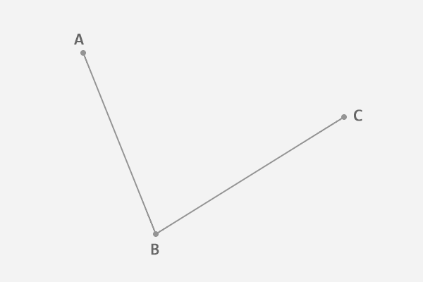
先在一个平面内任选 3 个不共线的点,依次用线段连接,如图:
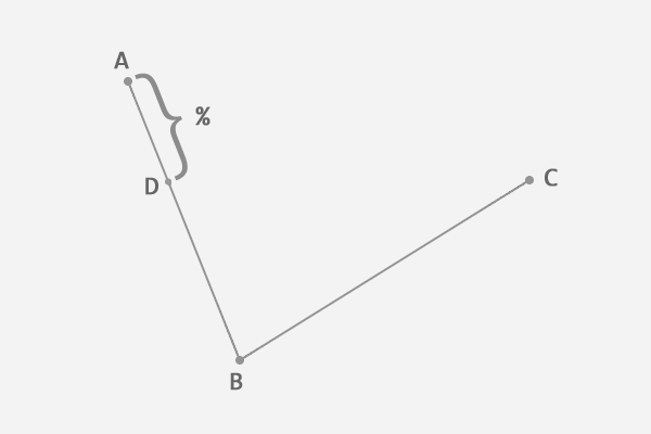
在第一条线段上任选一个点 D,计算该点到线段起点的距离 AD,与该线段总长 AB 的比例.
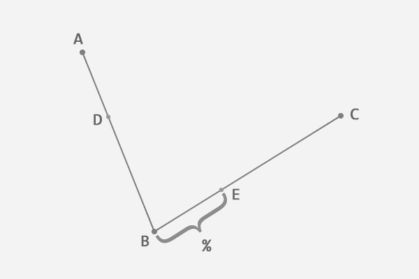
根据上一步得到的比例,从第二条线段上找出对应的点 E,使得 AD:AB = BE:BC.
连接这两点 DE.
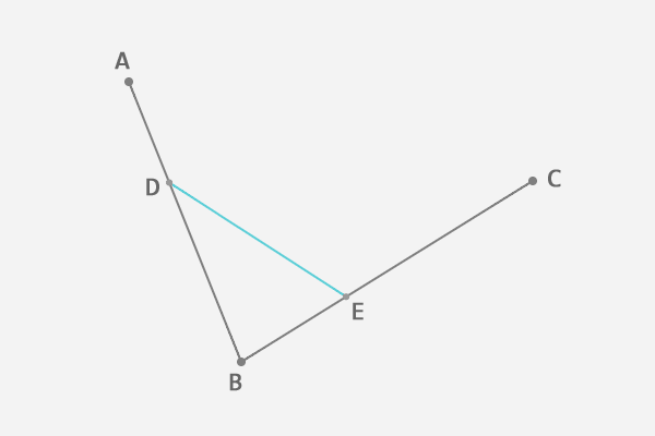
从新的线段 DE 上再次找出相同比例的点 F,使得 DF:DE = AD:AB=BE:BC.
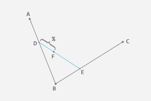
到这里,就确定了贝塞尔曲线上的一个点 F. 接下来,稍微回想一下中学所学的极限知识,让选取的点 D 在第一条线段上从起点 A 移动到终点 B,找出所有的贝塞尔曲线上的点 F. 所有的点找出来以后,也就得到了这条贝塞尔曲线.
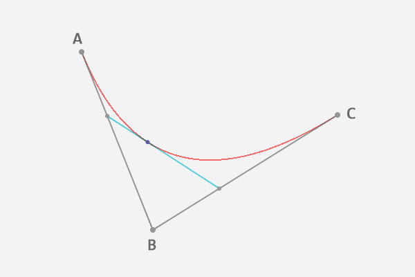
如果想象不出来,可以看下面的动画.

到这里,已经大概了解贝塞尔曲线绘制的过程了.
下面看公式.
2. 公式
以下公式中:
$B(t)$ 为 $t$ 时间下点的坐标;
$P_0$ 为起点;$P_n$ 为终点,$P_i$ 为控制点.
2.1. 一阶贝塞尔曲线
一阶贝塞尔曲线只有起点和终点,并没有控制点,所以绘制出来的图形仅仅只是一条直线,那么在时间 t 为 1 秒的情况下,其公式为:
$$ B(t) = (1 - t) P_0 + tP_1, t \in [0, 1] $$
意义:由 $P_0$ 至 $P_1$ 的连续点, 描述的一条线段.
2.2. 二阶贝塞尔曲线
二阶贝塞尔曲线只存在一个控制点,此时从起点到终点的线段发生变化,具体的变化是由控制点的位置而改变的. 图中,绿色的线段为红色曲线的切线.
$$ B(t) = (1 - t)^2 P_0 + 2t(1 - t)P_1 + t^2 P_2, t \in [0, 1] $$
仅仅只是简单的一元二次方程式.
原理:由 $P_0$ 至 $P_1$ 的连续点 $Q_0$,描述一条线段;由 $P_1$ 至 $P_2$ 的连续点 $Q_1$,描述一条线段;由 $Q_0$ 至 $Q_1$ 的连续点 $B(t)$,描述一条二次贝塞尔曲线.
Python 示例如:
#!/usr/bin/python3
#!--*-- coding: utf-8 --*--
import numpy as np
import matplotlib.pyplot as plt

P0, P1, P2 = np.array([[0, 0], [2, 4], [5, 3]])

# 定义贝塞尔曲线
P = lambda t: (1 - t)**2 * P0 + 2 * t * (1 - t) * P1 + t**2 * P2

# 在 [0, 1] 范围内的 50 个点上验证贝塞尔曲线
points = np.array([P(t) for t in np.linspace(0, 1, 50)])

# 分别获取点的 x 坐标和 y 坐标
x, y = points[:, 0], points[:, 1]

#
plt.plot(x, y, 'b-')
plt.plot(*P0, 'r.')
plt.plot(*P1, 'r.')
plt.plot(*P2, 'r.')
plt.show()
如:
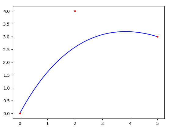
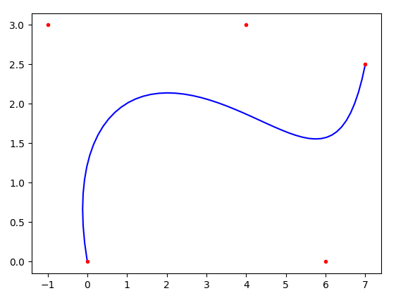
可以看到,曲线从第一个控制点处开始,到最后一个控制点处结束. 这个结果对任意数量的点都成立.
从P0到P2,P1 完全决定了曲线的形状。移动 P1:
贝塞尔曲线总是包含在控制点形成的多边形中. 这个多边形因此被称为控制多边形,或者贝塞尔多边形. 这个属性也适用于任意数量的控制点,这使得它们在使用软件时的操作非常直观.
控制多边形还具有以下特性:包含曲线的面积最小,称为凸包.
2.3. 高阶贝塞尔曲线
[1] - 三阶
[2] - 四阶
[3] - 五阶
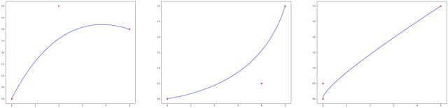
从三阶开始贝塞尔曲线就开始显得复杂了,高阶的通用公式如下:
$$ P_i^k = (1 - t) P_i^{k-1} + t P_{i+1}^{k-1} $$
其中,$k = 1, 2, ..., n$,$i = 0, 1, ..., n-k$.
https://pages.mtu.edu/~shene/COURSES/cs3621/NOTES/spline/Bezier/de-casteljau.html
任意数量的控制点贝塞尔曲线的 Python 实现:
#!/usr/bin/python3
#!--*-- coding: utf-8 --*--
import numpy as np
import matplotlib.pyplot as plt
from math import factorial

def comb(n, k):
    return factorial(n) // (factorial(k) * factorial(n-k))

def get_bezier_curve(points):
    n = len(points) - 1
    return lambda t: sum(comb(n, i)*t**i * (1-t)**(n-i)*points[i] for i in range(n+1))

def evaluate_bezier(points, total):
    bezier = get_bezier_curve(points)
    new_points = np.array([bezier(t) for t in np.linspace(0, 1, total)])
    return new_points[:, 0], new_points[:, 1]

points = np.array([[0, 0], [-1, 3], [4, 3], [6, 0], [7, 2.5]])
x, y = points[:, 0], points[:, 1]
bx, by = evaluate_bezier(points, 50)
#
plt.plot(bx, by, 'b-')
plt.plot(x, y, 'r.')
plt.show()
如图:
3. 插值
贝塞尔曲线的一个有趣应用是绘制一条通过一组预定义点的平滑曲线。之所以有趣,是因为 $P(t)$ 的公式产生点,并且不是 $y = f(x)$ 的形式,因此一个 $x$ 有多个 $y$. 例如,可以这样画:
贝塞尔插值实现如:
From: Bézier Interpolation - Create smooth shapes using Bézier curves - 2020.05.09
#!/usr/bin/python3
#!--*-- coding: utf-8 --*--
import numpy as np
import matplotlib.pyplot as plt

# find the a & b points
def get_bezier_coef(points):
    # since the formulas work given that we have n+1 points
    # then n must be this:
    n = len(points) - 1

    # build coefficents matrix
    C = 4 * np.identity(n)
    np.fill_diagonal(C[1:], 1)
    np.fill_diagonal(C[:, 1:], 1)
    C[0, 0] = 2
    C[n - 1, n - 1] = 7
    C[n - 1, n - 2] = 2

    # build points vector
    P = [2 * (2 * points[i] + points[i + 1]) for i in range(n)]
    P[0] = points[0] + 2 * points[1]
    P[n - 1] = 8 * points[n - 1] + points[n]

    # solve system, find a & b
    A = np.linalg.solve(C, P)
    B = [0] * n
    for i in range(n - 1):
        B[i] = 2 * points[i + 1] - A[i + 1]
    B[n - 1] = (A[n - 1] + points[n]) / 2

    return A, B

# returns the general Bezier cubic formula given 4 control points
def get_cubic(a, b, c, d):
    return lambda t: np.power(1 - t, 3) * a + 3 * np.power(1 - t, 2) * t * b + 3 * (1 - t) * np.power(t, 2) * c + np.power(t, 3) * d

# return one cubic curve for each consecutive points
def get_bezier_cubic(points):
    A, B = get_bezier_coef(points)
    return [
        get_cubic(points[i], A[i], B[i], points[i + 1])
        for i in range(len(points) - 1)
    ]

# evalute each cubic curve on the range [0, 1] sliced in n points
def evaluate_bezier(points, n):
    curves = get_bezier_cubic(points)
    return np.array([fun(t) for fun in curves for t in np.linspace(0, 1, n)])

#
# generate 5 (or any number that you want) random points that we want to fit (or set them youreself)
points = np.random.rand(5, 2)

# fit the points with Bezier interpolation
# use 50 points between each consecutive points to draw the curve
path = evaluate_bezier(points, 50)

# extract x & y coordinates of points
x, y = points[:,0], points[:,1]
px, py = path[:,0], path[:,1]

# plot
plt.figure(figsize=(11, 8))
plt.plot(px, py, 'b-')
plt.plot(x, y, 'ro')
plt.show()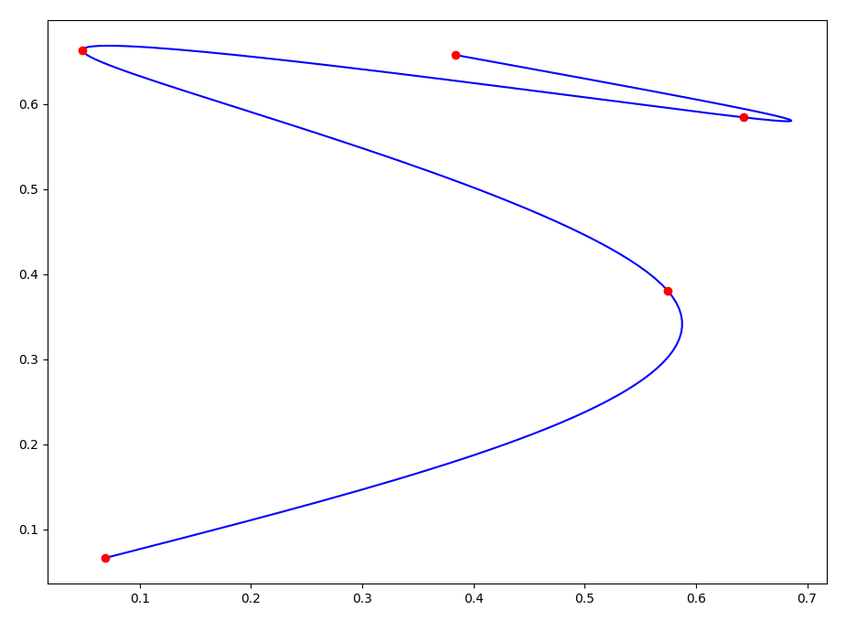
4. 三阶贝塞尔曲线插值平滑
From: python基于三阶贝塞尔曲线的数据平滑算法 - 2019.12.27
很多文章在谈及曲线平滑的时候,习惯使用拟合的概念,可能不太不恰当的. 平滑后的曲线,一定经过原始的数据点,而拟合曲线,则不一定要经过原始数据点.
一般而言,需要平滑的数据分为两种:时间序列的单值数据和时间序列的二维数据. 对于前者,并非一定要用贝塞尔算法,仅用样条插值就可以轻松实现平滑;而对于后者,不管是 numpy 还是 scipy 提供的那些插值算法,就都不适用了.
基于三阶贝塞尔曲线,实现时间序列的单值数据和时间序列的二维数据的平滑算法,可满足大多数的平滑需求。
4.1. 算法描述
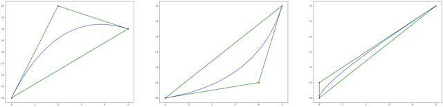
如果把三阶贝塞尔曲线的 P0 和 P3 视为原始数据,只要找到 P1 和 P2 两个点(称其为控制点),就可以根据三阶贝塞尔曲线公式,计算出 P0 和 P3 之间平滑曲线上的任意点。
现在,平滑问题变成了如何计算两个原始数据点之间的控制点的问题。步骤如下:
[1] - 绿色直线连接相邻的原始数据点,计算出个线段的中点,红色直线连接相邻的中点
[2] - 根据相邻两条绿色直线长度之比,分割其中点之间红色连线,标记分割点
[3] - 平移红色连线,使其分割点与相对的原始数据点重合
[4] - 调整平移后红色连线的端点与原始数据点的距离,通常缩减40%-80%

4.2. Python 实现
# !/usr/bin/python3
# !--*-- coding: utf-8 --*--
import numpy as np
import matplotlib.pyplot as plt
def bezier_curve(p0, p1, p2, p3, inserted):
"""
三阶贝塞尔曲线
p0, p1, p2, p3 - 点坐标,tuple、list或numpy.ndarray类型
inserted - p0和p3之间插值的数量
"""
assert isinstance(p0, (tuple, list, np.ndarray))
assert isinstance(p0, (tuple, list, np.ndarray))
assert isinstance(p0, (tuple, list, np.ndarray))
assert isinstance(p0, (tuple, list, np.ndarray))
if isinstance(p0, (tuple, list)):
p0 = np.array(p0)
if isinstance(p1, (tuple, list)):
p1 = np.array(p1)
if isinstance(p2, (tuple, list)):
p2 = np.array(p2)
if isinstance(p3, (tuple, list)):
p3 = np.array(p3)
points = list()
for t in np.linspace(0, 1, inserted + 2):
points.append(p0 * np.power((1 - t), 3) + 3 * p1 * t * np.power((1 - t), 2) + 3 * p2 * (1 - t) * np.power(t,
2) + p3 * np.power(
t, 3))
return np.vstack(points)
def smoothing_base_bezier(date_x, date_y, k=0.5, inserted=10, closed=False):
"""
基于三阶贝塞尔曲线的数据平滑算法
date_x - x维度数据集,list或numpy.ndarray类型
date_y - y维度数据集,list或numpy.ndarray类型
k - 调整平滑曲线形状的因子,取值一般在0.2~0.6之间。默认值为0.5
inserted - 两个原始数据点之间插值的数量。默认值为10
closed - 曲线是否封闭,如是,则首尾相连。默认曲线不封闭
"""
assert isinstance(date_x, (list, np.ndarray))
assert isinstance(date_y, (list, np.ndarray))
if isinstance(date_x, list) and isinstance(date_y, list):
assert len(date_x) == len(date_y), u'x数据集和y数据集长度不匹配'
date_x = np.array(date_x)
date_y = np.array(date_y)
elif isinstance(date_x, np.ndarray) and isinstance(date_y, np.ndarray):
assert date_x.shape == date_y.shape, u'x数据集和y数据集长度不匹配'
else:
raise Exception(u'x数据集或y数据集类型错误')
# 第1步:生成原始数据折线中点集
mid_points = list()
for i in range(1, date_x.shape[0]):
mid_points.append({
'start': (date_x[i - 1], date_y[i - 1]),
'end': (date_x[i], date_y[i]),
'mid': ((date_x[i] + date_x[i - 1]) / 2.0, (date_y[i] + date_y[i - 1]) / 2.0)
})
if closed:
mid_points.append({
'start': (date_x[-1], date_y[-1]),
'end': (date_x[0], date_y[0]),
'mid': ((date_x[0] + date_x[-1]) / 2.0, (date_y[0] + date_y[-1]) / 2.0)
})
# 第2步:找出中点连线及其分割点
split_points = list()
for i in range(len(mid_points)):
if i < (len(mid_points) - 1):
j = i + 1
elif closed:
j = 0
else:
continue
x00, y00 = mid_points[i]['start']
x01, y01 = mid_points[i]['end']
x10, y10 = mid_points[j]['start']
x11, y11 = mid_points[j]['end']
d0 = np.sqrt(np.power((x00 - x01), 2) + np.power((y00 - y01), 2))
d1 = np.sqrt(np.power((x10 - x11), 2) + np.power((y10 - y11), 2))
k_split = 1.0 * d0 / (d0 + d1)
mx0, my0 = mid_points[i]['mid']
mx1, my1 = mid_points[j]['mid']
split_points.append({
'start': (mx0, my0),
'end': (mx1, my1),
'split': (mx0 + (mx1 - mx0) * k_split, my0 + (my1 - my0) * k_split)
})
# 第3步:平移中点连线,调整端点,生成控制点
crt_points = list()
for i in range(len(split_points)):
vx, vy = mid_points[i]['end'] # 当前顶点的坐标
dx = vx - split_points[i]['split'][0] # 平移线段x偏移量
dy = vy - split_points[i]['split'][1] # 平移线段y偏移量
sx, sy = split_points[i]['start'][0] + dx, split_points[i]['start'][1] + dy # 平移后线段起点坐标
ex, ey = split_points[i]['end'][0] + dx, split_points[i]['end'][1] + dy # 平移后线段终点坐标
cp0 = sx + (vx - sx) * k, sy + (vy - sy) * k # 控制点坐标
cp1 = ex + (vx - ex) * k, ey + (vy - ey) * k # 控制点坐标
if crt_points:
crt_points[-1].insert(2, cp0)
else:
crt_points.append([mid_points[0]['start'], cp0, mid_points[0]['end']])
if closed:
if i < (len(mid_points) - 1):
crt_points.append([mid_points[i + 1]['start'], cp1, mid_points[i + 1]['end']])
else:
crt_points[0].insert(1, cp1)
else:
if i < (len(mid_points) - 2):
crt_points.append([mid_points[i + 1]['start'], cp1, mid_points[i + 1]['end']])
else:
crt_points.append([mid_points[i + 1]['start'], cp1, mid_points[i + 1]['end'], mid_points[i + 1]['end']])
crt_points[0].insert(1, mid_points[0]['start'])
# 第4步:应用贝塞尔曲线方程插值
out = list()
for item in crt_points:
group = bezier_curve(item[0], item[1], item[2], item[3], inserted)
out.append(group[:-1])
out.append(group[-1:])
out = np.vstack(out)
return out.T[0], out.T[1]
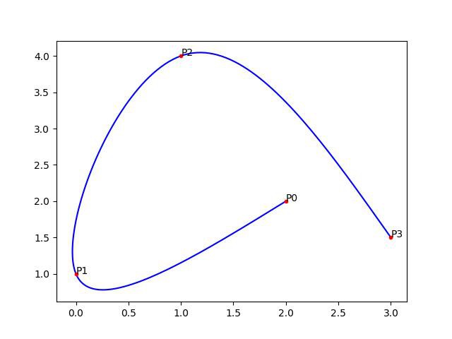
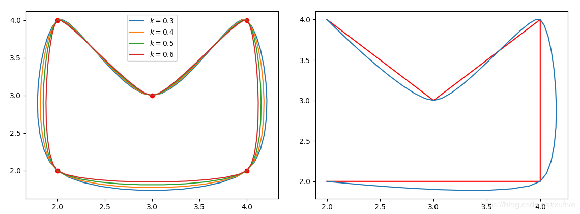
if __name__ == '__main__':
x = np.array([2, 4, 4, 3, 2])
y = np.array([2, 2, 4, 3, 4])
plt.plot(x, y, 'ro')
x_curve, y_curve = smoothing_base_bezier(x, y, k=0.3, closed=True)
plt.plot(x_curve, y_curve, label='$k=0.3$')
x_curve, y_curve = smoothing_base_bezier(x, y, k=0.4, closed=True)
plt.plot(x_curve, y_curve, label='$k=0.4$')
x_curve, y_curve = smoothing_base_bezier(x, y, k=0.5, closed=True)
plt.plot(x_curve, y_curve, label='$k=0.5$')
x_curve, y_curve = smoothing_base_bezier(x, y, k=0.6, closed=True)
plt.plot(x_curve, y_curve, label='$k=0.6$')
plt.legend(loc='best')
plt.show()下图为平滑效果。左侧是封闭曲线,两个原始数据点之间插值数量为默认值10;右侧为同样数据不封闭的效果,k值默认0.5.
材料
[1] - 关于贝塞尔曲线的公式推导和python代码实现 - 2020.09.27 - 知乎
[2] - 了解贝塞尔曲线的数学和Python实现示例 - 2020.05.03
[3] - Bézier Interpolation - Create smooth shapes using Bézier curves - 2020.05.09
[4] - python基于三阶贝塞尔曲线的数据平滑算法 - 2019.12.27
[5] - Interpolation with Bezier Curves - A very simple method of smoothing polygons
[6] - 贝塞尔曲线 - 百度百科
3 条评论
好的工作,爱来自中国
NICE,超级棒⌇●﹏●⌇
(☆ω☆) nice !