原文:Multi-Label Image Classification with PyTorch: Image Tagging - 2020.05.03
作者:Victor Bebnev (Xperience.AI)
实现:Github - PyTorch-Multi-Label-Image-Classification-Image-Tagging
在 图像标注-基于PyTorch的多输出图像分类 中,主要是针对每张图片输出固定数量标签的场景(mult-outputs).
1. 多标签分类
首先,明确下多标签分类(multi-label classification) 的定义,以及其与多类别分类(multi-class classification) 的区别.
根据 scikit-learn 中所述,multi-label 分类是对每个样本分配一组目标标签集;而,multi-class 分类是假设每个样本仅有目标标签集中的一个标签. 此外,multi-label 分类中,每个样本的所有标签不是互斥的(mutually exclusive).
在 Multi-Label Image Classification with PyTorch 中,是 multi-output 的分类问题,其处理的也是每个样本多个标签的分类问题. multi-output 分类问题,其往往预测的是每个样本的固定数量的标签;且,理论上可以由相应输出标签数量的独立分类器来替代. 而,multi-label 分类问题往往需要预测非固定数量的标签.multi-output 分类问题必须知道有几个独立的问题,每个问题有且仅有一个可能的答案.
为了总结不同分类任务间(multi-class、multi-output、multi-label)的差异性,以下图为例说明.

图-标签可以是:portrait, woman, smiling, brown hair, wavy hair
| Type | Predicted labels | Possible labels |
|---|---|---|
| Multi-class classification | smiling | [neutral, smiling, sad] |
| Multi-output classification | woman, smiling, brown hair | [man, woman, child] [neutral, smiling, sad] [brown hair, red hair, blond hair, black hair] |
| Multi-label classification | portrait, woman, smiling, brown hair, wavy hair | [portrait, nature, landscape, selfie, man, woman, child, neutral emotion, smiling, sad, brown hair, red hair, blond hair, black hair] |
在现实生活中,比如 Instagram 标签,用户往往是从标签池里选择某些标签对图片进行标注(为了举例说明,这里假设标签池是固定的). 这些标签往往不是互斥的,它们表征的是图片里所刻画的特征,如“woman”, “wavy hair”, “smiling girl”, “cool shirt”;或者更高层次的语义,如 “portrait”, “happiness”, “fun”.
下面以 NUS-WIDE 数据集为例进行说明.
2. 数据集
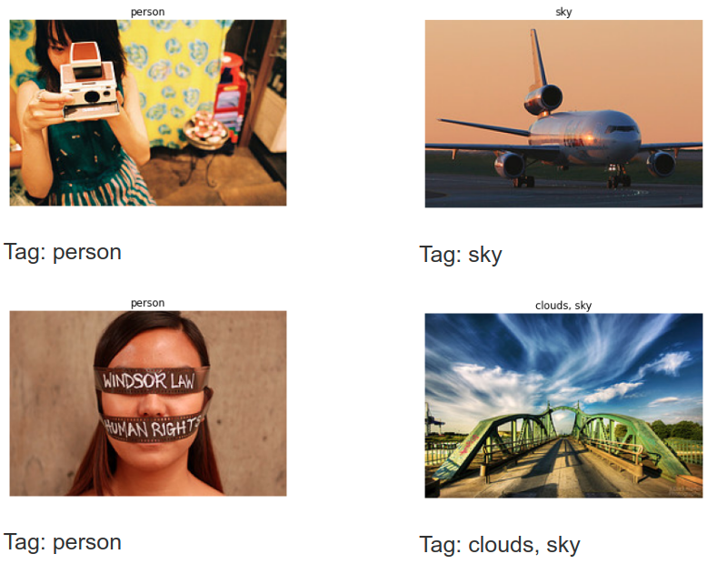
这里采用 NUS-WIDE 数据集中的一部分. 该数据集每张图片被标注了多个标签. 其图片收集自 Flickr,包含了超过 1000 个不同标签,最终被收窄到 81 个. 例如,
2.1. 数据集划分
NUS-WIDE 数据集共包含约 170K 个样本,其标签是高度不均衡的. 例如,对于某些标签,如 sky 和 clouds,数量量约 61000 和 45000;而对于其它标签,如 map 和 earthquake,数量仅为 50.
鉴于这里的主要目的是阐述如何处理 multi-label 分类问题,所以将问题进行简化. 仅保留 27 个最频繁出现的标签,使得每个标签具有超过 100 个样本. 此外,为了快速模型训练,仅使用数据集中的前 6000 个样本. 并按照 5:1 来划分为 train 和 val 数据集. 最终得到训练数据集为 5000 张图片,测试数据集为 1000 张图片.
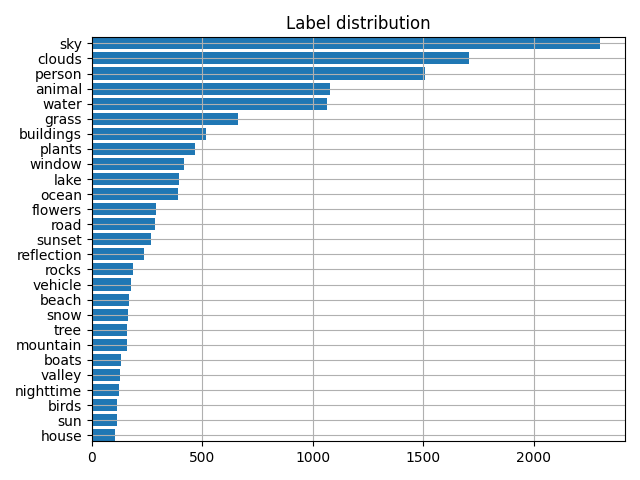 图- NUS-WIDE 数据集的标签分布.
2.2. 数据处理实现
每条标注数据格式类似于:
[
    'samples':
        [
            {'image_name': '51353_2739084573_16e9be31f5_m.jpg' , 'image_labels': ['clouds', 'sky']}
            ...
        ]
    'labels' : ['house', 'birds', 'sun', 'valley', 'nighttime', 'boats', ...]
]
代码实现:
import os
import time
import numpy as np
from PIL import Image
from torch.utils.data.dataset import Dataset
from tqdm import tqdm
from torchvision import transforms
from torchvision import models
import torch
from torch.utils.tensorboard import SummaryWriter
from sklearn.metrics import precision_score, recall_score, f1_score
from torch import nn
from torch.utils.data.dataloader import DataLoader
from matplotlib import pyplot as plt
from numpy import printoptions
import requests
import tarfile
import random
import json
from shutil import copyfile

# For reproducible
torch.manual_seed(2020)
torch.cuda.manual_seed(2020)
np.random.seed(2020)
random.seed(2020)
torch.backends.cudnn.deterministic = True

# 数据集下载
img_folder = 'images'
if not os.path.exists(img_folder):
    def download_file_from_google_drive(id, destination):
        def get_confirm_token(response):
            for key, value in response.cookies.items():
                if key.startswith('download_warning'):
                    return value
            return None

        def save_response_content(response, destination):
            CHUNK_SIZE = 32768
            with open(destination, "wb") as f:
                for chunk in tqdm(response.iter_content(CHUNK_SIZE), desc='Downloading'):
                    if chunk:  # filter out keep-alive new chunks
                        f.write(chunk)

        URL = "https://docs.google.com/uc?export=download"
        session = requests.Session()
        response = session.get(URL, params={'id': id}, stream=True)
        token = get_confirm_token(response)

        if token:
            params = {'id': id, 'confirm': token}
            response = session.get(URL, params=params, stream=True)
        save_response_content(response, destination)

    #
    file_id = '0B7IzDz-4yH_HMFdiSE44R1lselE'
    path_to_tar_file = str(time.time()) + '.tar.gz'
    download_file_from_google_drive(file_id, path_to_tar_file)
    print('Extraction')
    with tarfile.open(path_to_tar_file) as tar_ref:
        tar_ref.extractall(os.path.dirname(img_folder))
    os.remove(path_to_tar_file)
# Also, copy our pre-processed annotations to the dataset folder.
# Note: you can find script for generating such annotations in attachments
copyfile('nus_wide/small_test.json', os.path.join(img_folder, 'small_test.json'))
copyfile('nus_wide/small_train.json', os.path.join(img_folder, 'small_train.json'))

#
# 数据集加载
# Dataloader,标签二值化.
class NusDataset(Dataset):
    def __init__(self, data_path, anno_path, transforms):
        self.transforms = transforms
        with open(anno_path) as fp:
            json_data = json.load(fp)
        samples = json_data['samples']
        self.classes = json_data['labels']

        self.imgs = []
        self.annos = []
        self.data_path = data_path
        print('loading', anno_path)
        for sample in samples:
            self.imgs.append(sample['image_name'])
            self.annos.append(sample['image_labels'])
        for item_id in range(len(self.annos)):
            item = self.annos[item_id]
            vector = [cls in item for cls in self.classes]
            self.annos[item_id] = np.array(vector, dtype=float)

    def __getitem__(self, item):
        anno = self.annos[item]
        img_path = os.path.join(self.data_path, self.imgs[item])
        img = Image.open(img_path)
        if self.transforms is not None:
            img = self.transforms(img)
        return img, anno

    def __len__(self):
        return len(self.imgs)

# 数据集可视化
dataset_val = NusDataset(img_folder, os.path.join(img_folder, 'small_test.json'), None)
dataset_train = NusDataset(img_folder, os.path.join(img_folder, 'small_train.json'), None)

#
def show_sample(img, binary_img_labels):
    # Convert the binary labels back to the text representation.
    img_labels = np.array(dataset_val.classes)[np.argwhere(binary_img_labels > 0)[:, 0]]
    plt.imshow(img)
    plt.title("{}".format(', '.join(img_labels)))
    plt.axis('off')
    plt.show()

for sample_id in range(5):
    show_sample(*dataset_val[sample_id])

# 统计数据集的标签分布
samples = dataset_val.annos + dataset_train.annos
samples = np.array(samples)
with printoptions(precision=3, suppress=True):
    class_counts = np.sum(samples, axis=0)
    # Sort labels according to their frequency in the dataset.
    sorted_ids = np.array([i[0] for i in sorted(enumerate(class_counts), key=lambda x: x[1])], dtype=int)
    print('Label distribution (count, class name):', list(zip(class_counts[sorted_ids].astype(int), np.array(dataset_val.classes)[sorted_ids])))
    plt.barh(range(len(dataset_val.classes)), width=class_counts[sorted_ids])
    plt.yticks(range(len(dataset_val.classes)), np.array(dataset_val.classes)[sorted_ids])
    plt.gca().margins(y=0)
    plt.grid()
    plt.title('Label distribution')
    plt.show()
3. 创建模型
3.1. 模型结构
模型的 backbone 网络结构,采用 torchvision 中的 ResNeXt50 结构. 并修改其输出层,以适应 multi-label 分类任务.
不同的是,ResNeXt50 的标准输出为 1000 个类(ImageNet),而这里是 27 个. 此外,替换 softmax 函数为 sigmoid 函数. 后面会介绍原因.
class Resnext50(nn.Module):
    def __init__(self, n_classes):
        super().__init__()
        resnet = models.resnext50_32x4d(pretrained=True)
        resnet.fc = nn.Sequential(
            nn.Dropout(p=0.2),
            nn.Linear(in_features=resnet.fc.in_features, out_features=n_classes)
        )
        self.base_model = resnet
        self.sigm = nn.Sigmoid()

    def forward(self, x):
        return self.sigm(self.base_model(x))
3.2. 损失函数
在数据集确定及定义模型结构后,剩下的事情是选择损失函数. 由于是分类任务,其选择看似比较明显 - 交叉熵损失函数(CrossEntropy Loss). 但,这里会说明为什么其不适用于 multi-label 问题.
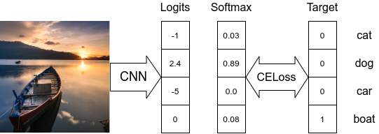
图 - 模型采用 Softmax 分类器及交叉熵损失函数.
上图给出了在各标签互斥的 multi-class 分类场景中交叉熵损失函数的计算. 在损失函数计算时,仅关注和 GT 标签对应的 logit,以及其与其它标签的差异性. 例如,上图中,损失函数值为: $-log(0.08)=2.52$
Softmax 函数会将所有预测结果的概率和置为 1,因此,其不能处理存在多个正确标签的情况.

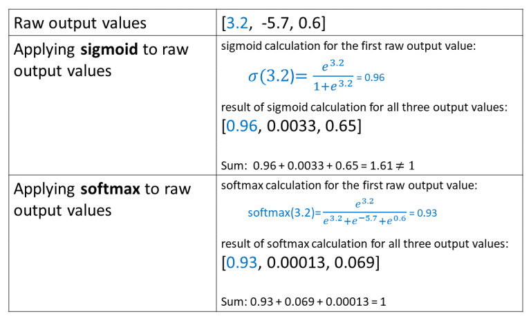
图 - 模型采用 Sigmoid 分类器
显而易见的方案是,将每个预测分别独立对待. 例如,采用 Sigmoid 函数对每个 logit 值分别归一化.
Multi-label 问题中,会存在多个正确标签以及每个标签对应的预测概率. 然后,即可采用 BinaryCrossEntropy 损失函数计算每个标签的概率和 GT 之间的偏差.

图 - 模型采用 Sigmoid 分类器和 BinaryCrossEntropyLoss.
因此,最终采用 BinaryCrossEntropy 损失函数.
criterion = nn.BCELoss()Sigmoid 和 Softmax 的计算对比:
至此,剩下的唯一问题就是,在预测截断如何处理预测的概率. 通用做法是设置阈值,如果输出标签的概率值大于阈值,则表示为预测标签,否则跳过. 这里设置阈值为 0.5.
3.3. 度量方式Metrics
采用 sklearn.metrics.precision_score 计算度量,其参数设定为 average='macro'、average='micro' 或 average='samples'.
def calculate_metrics(pred, target, threshold=0.5):
    pred = np.array(pred > threshold, dtype=float)
    return {'micro/precision': precision_score(y_true=target, y_pred=pred, average='micro'),
            'micro/recall': recall_score(y_true=target, y_pred=pred, average='micro'),
            'micro/f1': f1_score(y_true=target, y_pred=pred, average='micro'),
            'macro/precision': precision_score(y_true=target, y_pred=pred, average='macro'),
            'macro/recall': recall_score(y_true=target, y_pred=pred, average='macro'),
            'macro/f1': f1_score(y_true=target, y_pred=pred, average='macro'),
            'samples/precision': precision_score(y_true=target, y_pred=pred, average='samples'),
            'samples/recall': recall_score(y_true=target, y_pred=pred, average='samples'),
            'samples/f1': f1_score(y_true=target, y_pred=pred, average='samples'),
            }
3.4. 模型训练
实现如下:
# 初始化训练参数
num_workers = 8 # Number of CPU processes for data preprocessing
lr = 1e-4 # Learning rate
batch_size = 32
save_freq = 1 # Save checkpoint frequency (epochs)
test_freq = 200 # Test model frequency (iterations)
max_epoch_number = 35 # Number of epochs for training
# Note: on the small subset of data overfitting happens after 30-35 epochs

mean = [0.485, 0.456, 0.406]
std = [0.229, 0.224, 0.225]

device = torch.device('cuda')
# Save path for checkpoints
save_path = 'chekpoints/'
# Save path for logs
logdir = 'logs/'

# 辅助函数,断点保存
def checkpoint_save(model, save_path, epoch):
    f = os.path.join(save_path, 'checkpoint-{:06d}.pth'.format(epoch))
    if 'module' in dir(model):
        torch.save(model.module.state_dict(), f)
    else:
        torch.save(model.state_dict(), f)
    print('saved checkpoint:', f)

#数据处理
# Test preprocessing
val_transform = transforms.Compose([
    transforms.Resize((256, 256)),
    transforms.ToTensor(),
    transforms.Normalize(mean, std)
])
print(tuple(np.array(np.array(mean)*255).tolist()))

# Train preprocessing
train_transform = transforms.Compose([
    transforms.Resize((256, 256)),
    transforms.RandomHorizontalFlip(),
    transforms.ColorJitter(),
    transforms.RandomAffine(
        degrees=20,
        translate=(0.2, 0.2),
        scale=(0.5, 1.5),
        shear=None,
        resample=False,
        fillcolor=tuple(np.array(np.array(mean)*255).astype(int).tolist())),
    transforms.ToTensor(),
    transforms.Normalize(mean, std)
])


# Initialize the dataloaders for training.
test_annotations = os.path.join(img_folder, 'small_test.json')
train_annotations = os.path.join(img_folder, 'small_train.json')

test_dataset = NusDataset(img_folder, test_annotations, val_transform)
train_dataset = NusDataset(img_folder, train_annotations, train_transform)

train_dataloader = DataLoader(train_dataset, batch_size=batch_size, num_workers=num_workers, shuffle=True,
                              drop_last=True)
test_dataloader = DataLoader(test_dataset, batch_size=batch_size, num_workers=num_workers)

num_train_batches = int(np.ceil(len(train_dataset) / batch_size))

# Initialize the model
model = Resnext50(len(train_dataset.classes))
# Switch model to the training mode and move it to GPU.
model.train()
model = model.to(device)

optimizer = torch.optim.Adam(model.parameters(), lr=lr)

# If more than one GPU is available we can use both to speed up the training.
if torch.cuda.device_count() > 1:
    model = nn.DataParallel(model)

os.makedirs(save_path, exist_ok=True)

# Loss function
criterion = nn.BCELoss()
# Tensoboard logger
logger = SummaryWriter(logdir)


# Run training
epoch = 0
iteration = 0
while True:
    batch_losses = []
    for imgs, targets in train_dataloader:
        imgs, targets = imgs.to(device), targets.to(device)

        optimizer.zero_grad()

        model_result = model(imgs)
        loss = criterion(model_result, targets.type(torch.float))

        batch_loss_value = loss.item()
        loss.backward()
        optimizer.step()

        logger.add_scalar('train_loss', batch_loss_value, iteration)
        batch_losses.append(batch_loss_value)
        with torch.no_grad():
            result = calculate_metrics(model_result.cpu().numpy(), targets.cpu().numpy())
            for metric in result:
                logger.add_scalar('train/' + metric, result[metric], iteration)

        if iteration % test_freq == 0:
            model.eval()
            with torch.no_grad():
                model_result = []
                targets = []
                for imgs, batch_targets in test_dataloader:
                    imgs = imgs.to(device)
                    model_batch_result = model(imgs)
                    model_result.extend(model_batch_result.cpu().numpy())
                    targets.extend(batch_targets.cpu().numpy())

            result = calculate_metrics(np.array(model_result), np.array(targets))
            for metric in result:
                logger.add_scalar('test/' + metric, result[metric], iteration)
            print("epoch:{:2d} iter:{:3d} test: "
                  "micro f1: {:.3f} "
                  "macro f1: {:.3f} "
                  "samples f1: {:.3f}".format(epoch, iteration,
                                              result['micro/f1'],
                                              result['macro/f1'],
                                              result['samples/f1']))

            model.train()
        iteration += 1
    #
    loss_value = np.mean(batch_losses)
    print("epoch:{:2d} iter:{:3d} train: loss:{:.3f}".format(epoch, iteration, loss_value))
    if epoch % save_freq == 0:
        checkpoint_save(model, save_path, epoch)
    epoch += 1
    if max_epoch_number < epoch:
        break
在 1080Ti 显卡上训练约 1 个小时,35 个 epochs直到过拟合. 最高 macro F1-score 为 0.520,其对应的最佳 micro F1-score 为 0.666. 存在的差异性的原因可能是数据相当不均衡所导致.
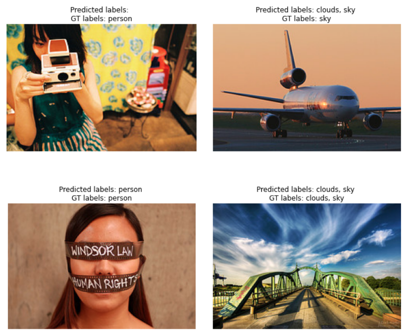
3.5. 模型预测
# Run inference on the test data
model.eval()
for sample_id in [1,2,3,4,6]:
    test_img, test_labels = test_dataset[sample_id]
    test_img_path = os.path.join(img_folder, test_dataset.imgs[sample_id])
    with torch.no_grad():
        raw_pred = model(test_img.unsqueeze(0)).cpu().numpy()[0]
        raw_pred = np.array(raw_pred > 0.5, dtype=float)

    predicted_labels = np.array(dataset_val.classes)[np.argwhere(raw_pred > 0)[:, 0]]
    if not len(predicted_labels):
        predicted_labels = ['no predictions']
    img_labels = np.array(dataset_val.classes)[np.argwhere(test_labels > 0)[:, 0]]
    plt.imshow(Image.open(test_img_path))
    plt.title("Predicted labels: {} \nGT labels: {}".format(', '.join(predicted_labels), ', '.join(img_labels)))
    plt.axis('off')
    plt.show()
如图:
4. 总结
这里主要简单介绍了关于 multi-label 分类问题的解决方案.
后面可以尝试更多 SoTA 论文,以及不同的损失函数、额外的处理等,以提升精度. 例如,使用当前热门的 GCN 为网络提供标签间的组合关系等信息,可能更合适.
5. 相关资料
[1] - Multi-Label Text Classification
[2] - Deep dive into multi-label classification
[3] - Multi-label vs. Multi-class Classification: Sigmoid vs. Softmax
4 条评论
small_test.json和small_train.json可以提供一下吗?
https://docs.google.com/uc?export=download这个url失效了怎么办
赞,学会了用PyTorch搭建图片多标签分类的pipeline
0.5的f1你为什么要发。。。