原文:使用 Python 通过基于颜色的图像分割进行物体检测 - 2019.04.15
出处:雷锋字幕组 - AI 研习社 微信公众号
英文:Object detection via color-based image segmentation using python
作者:Salma Ghoneim
主要参考自 使用 Python 通过基于颜色的图像分割进行物体检测 - AI 研习社的微信公众号文章.
这里关注与实现过程和验证是否有效.
1. 两个术语
[1] - 轮廓
轮廓可以简单地解释为连接所有连续点(连同边界)的曲线,具有相同的颜色或亮度.
轮廓是形状分析和目标检测和识别的有用工具。
[2] - 阈值
在灰度图像上应用阈值处理使其成为二值图像.
可以设置一个阈值,其中低于此阈值的所有值都将变为黑色,高于此阈值的所有值都将变为白色.
2. 简单例示
从一个简单的例子开始,展示基于颜色的分割是如何工作的.
如下图:
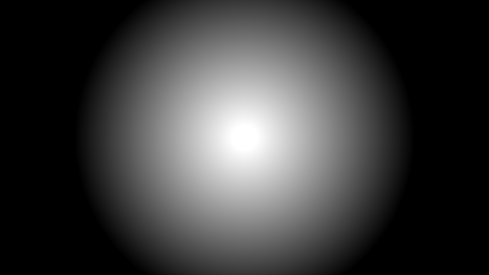
图1 - 一个Ombre圈 - 使用photoshop制作的图像
2.1. Step1 - 划分灰度级
采用下面的代码,将该图像分为 17 个灰度级,再使用轮廓来测量每个灰度级的区域.
#!/usr/bin/python3
#!--*-- coding: utf-8 --*--

import cv2
import numpy as np
import matplotlib.pyplot as plt


def grayscale_17_levels(gray_img):
    high = 255
    while (1):
        low = high - 15
        col_to_be_changed_low = np.array([low])
        col_to_be_changed_high = np.array([high])
        curr_mask = cv2.inRange(gray_img, col_to_be_changed_low, col_to_be_changed_high)
        gray_img[curr_mask > 0] = (high)
        high -= 15
        if (low == 0):
            break

    return  gray_img


img_file = "test.png"
img_cv2 = cv2.imread(img_file)

gray_img = cv2.cvtColor(img_cv2, cv2.COLOR_BGR2GRAY)
gray_img = grayscale_17_levels(gray_img)

plt.figure(figsize=(10, 8))
plt.subplot(1, 2, 1)
plt.imshow(img_cv2)
plt.title("Original image")
plt.axis("off")
plt.subplot(1, 2, 2)
plt.imshow(gray_img)
plt.title("Grayscale 17 levels image")
plt.axis("off")
plt.show()

print("Done.")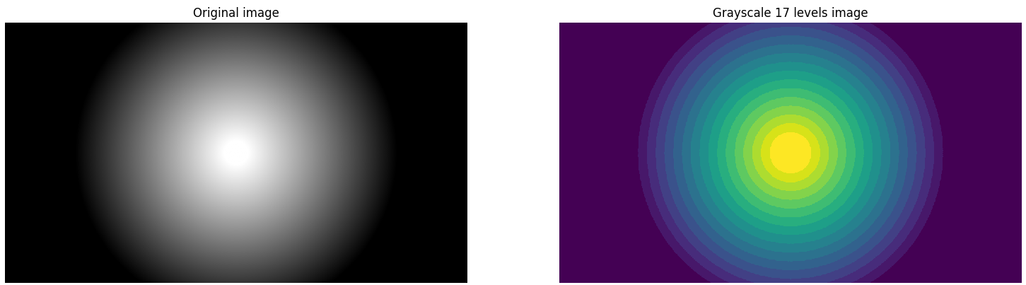

图2 - (右) 图像被分为 17 个灰度级
2.2. Step2 - 图像阈值化
定义如下函数,其作用只是通过将位于此范围内的所有数据统一到一个强度,在此迭代中简单地转换希望的轮廓(高亮)的灰色范围(强度). 这里将所有其他强度转换为黑色(包括更大和更小的强度).
def get_area_of_each_gray_level(im):
    # 在得到轮廓前,必须将图片转换为灰度图(gray scale)
    image = cv2.cvtColor(im, cv2.COLOR_BGR2GRAY)
    output = []
    high = 255
    first = True
    while (1):
        low = high - 15
        if (first == False):
            # 使得大于灰度级(gray level) 的值为 black,以便于不会被检测到.
            to_be_black_again_low = np.array([high])
            to_be_black_again_high = np.array([255])
            curr_mask = cv2.inRange(image, to_be_black_again_low, to_be_black_again_high)
            image[curr_mask > 0] = (0)

        # 使得当前灰度级的值为 white,以便于计算其面积
        ret, threshold = cv2.threshold(image, low, 255, 0)
        contours, hirerchy = cv2.findContours(threshold,
                                              cv2.RETR_LIST,
                                              cv2.CHAIN_APPROX_NONE)
        if (len(contours) > 0):
            output.append([cv2.contourArea(contours[0])])
        cv2.drawContours(im, contours, -1, (0, 0, 255), 3)
        high -= 15
        first = False
        if (low == 0):
            break

return output对图像进行阈值处理,以便只有想要轮廓的颜色现在显示为白色而其他所有颜色都转换为黑色.
此步骤在这里没有太大变化,但必须完成,因为轮廓最适合黑白(阈值)图像.
在阈值化处理之前,下面的图像将是相同的,除了白色环将变成灰色的(第10个灰度级的灰度强度(255-15 * 10)).

图 3 - 第10个灰度级部分单独出现以便能够计算其面积
image = cv2.imread('test.png')
print(get_area_of_each_gray_level(image))
plt.figure(figsize=(8, 6))
plt.imshow(image)
plt.axis("off")
plt.show()
输出:
#包含区域值的数组
[[5871.0], [6480.0], [13012.0], [21820.0], [32902.0], [46238.0], [61761.0], [79709.0], [99787.0], [122222.0], [146859.0], [173758.0], [202919.5], [234401.5], [12241.5], [11577.0], [11111.0]]
图 4 - 原始图像上的 17个灰度级的轮廓
即可得到每个灰度级的面积.
3. 重要性说明
这里强调下重要性,作者正在开展的一个名为机器学习的项目,用于智能肿瘤检测和识别.
该项目中使用基于颜色的图像分割来帮助计算机学习如何检测肿瘤. 当处理MRI扫描时,程序必须检测所述 MRI 扫描的癌症水平. 它通过将扫描分割成不同的灰度级别来实现这一点,其中最暗的是充满癌细胞,而最接近白色的是更健康的部分. 然后它计算肿瘤对每个灰度级的隶属程度. 有了这些信息,该程序能够识别肿瘤及其阶段.
该项目基于软计算,模糊逻辑和机器学习( soft computing, fuzzy logic & machine learning),可以在模糊逻辑及其如何治愈癌症方面了解更多信息.
4. 物体检测
以下图为例:
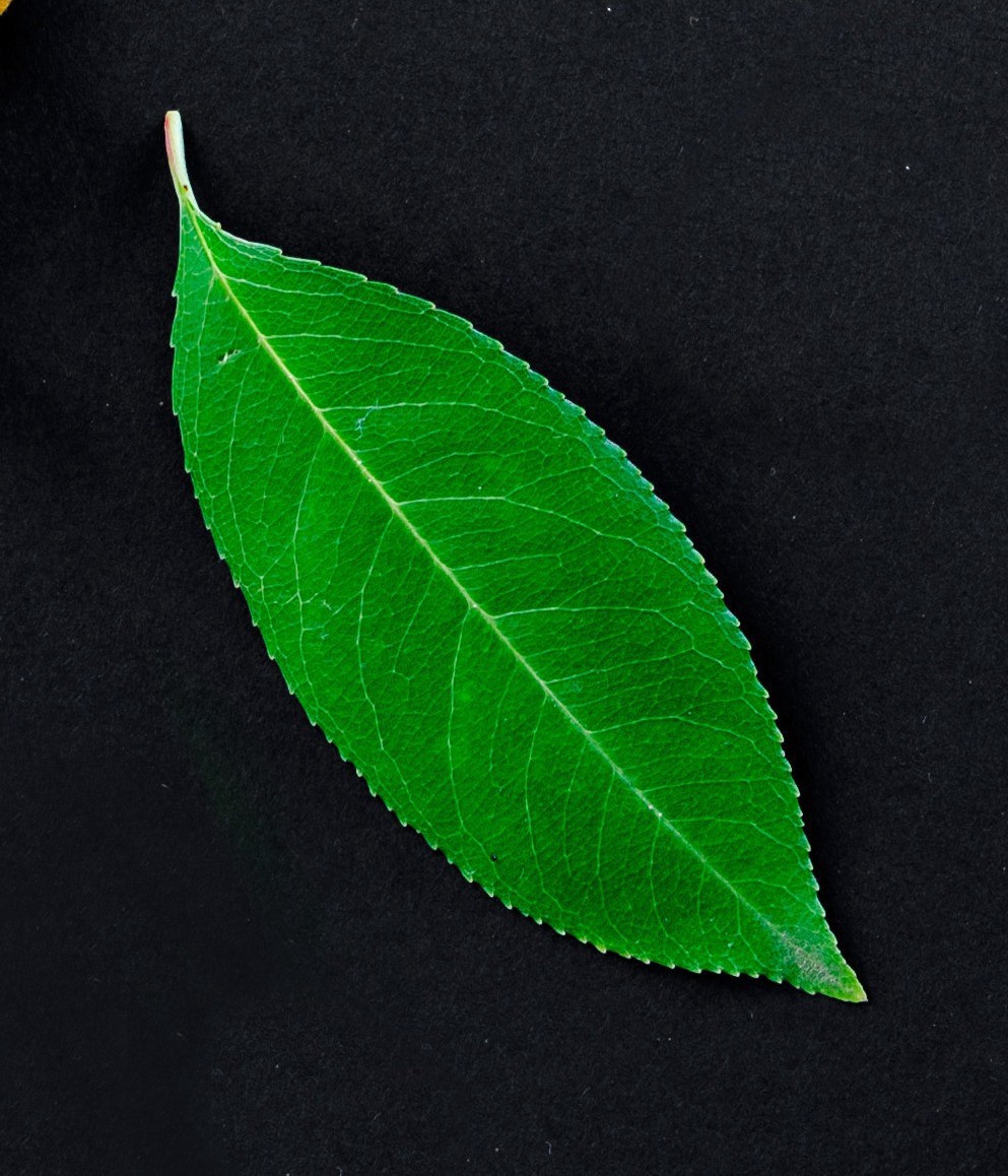
图5 - 例示图. Photo by Lukas from Pexels
对于此图像,目的是只想得到轮廓化叶子. 由于该图像的纹理非常不规则且不均匀,这意味着虽然没有很多颜色. 该图像中的绿色强度也能改变其亮度. 因此,这里最好的做法是将所有这些不同的绿色阴影统一为一个阴影. 这样当应用轮廓时,它将把叶子作为一个整体对象来处理。
注意:如果在图像上应用轮廓线而不进行任何预处理,则会出现以下情况. 这里只是想说明叶子的不均匀性如何让OpenCV识别不出这只是一个对象.
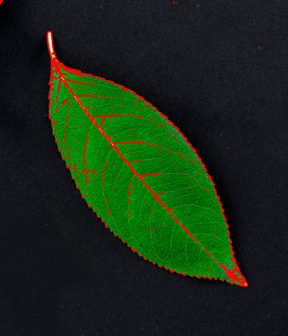
图6 - 在没有预处理的情况下进行轮廓加工,检测到531个轮廓.
4.1. 颜色的 HSV 表示
首先,必须知道颜色的HSV表示,可以通过将其RGB转换为HSV来了解它,如下所示:
import numpy as np
import cv2

#计算 green 的 HSV 颜色表示
green = np.uint8([[[0, 255, 0 ]]])
green_hsv = cv2.cvtColor(green,cv2.COLOR_BGR2HSV)
print(green_hsv)
输出:
#HSV颜色的绿色表示
[[[ 60 255 255]]]将图像转换为HSV:使用HSV可以更轻松地获得一种颜色的完整范围.
HSV,H代表Hue,S代表饱和度,V代表值.
4.2. 物体检测
已经知道绿色是 [60,255,255]. 世界上所有的绿色都在 [45,100,50] 到 [75,255,255] 之间,即[60-15,100,50]到 [60 + 15,255,255]. 15仅是近似值.
取这个范围并将其转换为[75,255,200]或任何其他浅色(第三个值必须相对较大),因为这是颜色的亮度,这是当到达阈值时使该部分为白色的值图片.
import cv2
import matplotlib.pyplot as plt

image = cv2.imread('test.jpeg')
plt.figure(figsize=(10, 8))
plt.subplot(2, 3, 1)
plt.imshow(image[:,:,::-1])
plt.axis("off")
plt.title("Original image")

hsv_img = cv2.cvtColor(image, cv2.COLOR_BGR2HSV)
plt.subplot(2, 3, 2)
plt.imshow(hsv_img[:,:,::-1])
plt.axis("off")
plt.title("hsv image")

green_low = np.array([45 , 100, 50] )
green_high = np.array([75, 255, 255])
curr_mask = cv2.inRange(hsv_img, green_low, green_high)
hsv_img[curr_mask > 0] = ([75,255,200])
plt.subplot(2, 3, 3)
plt.imshow(hsv_img[:,:,::-1])
plt.axis("off")
plt.title("hsv image")

## converting the HSV image to Gray inorder to be able to apply contouring
RGB_again = cv2.cvtColor(hsv_img, cv2.COLOR_HSV2RGB)
gray = cv2.cvtColor(RGB_again, cv2.COLOR_RGB2GRAY)
plt.subplot(2, 3, 4)
plt.imshow(gray)
plt.axis("off")
plt.title("gray image")

ret, threshold = cv2.threshold(gray, 90, 255, 0)
plt.subplot(2, 3, 5)
plt.imshow(threshold)
plt.axis("off")
plt.title("threshold image")

contours, hierarchy =  cv2.findContours(threshold,cv2.RETR_TREE,cv2.CHAIN_APPROX_SIMPLE)
cv2.drawContours(image, contours, -1, (0, 0, 255), 3)
plt.subplot(2, 3, 6)
plt.imshow(image[:,:,::-1])
plt.axis("off")
plt.title("contours image")

plt.show()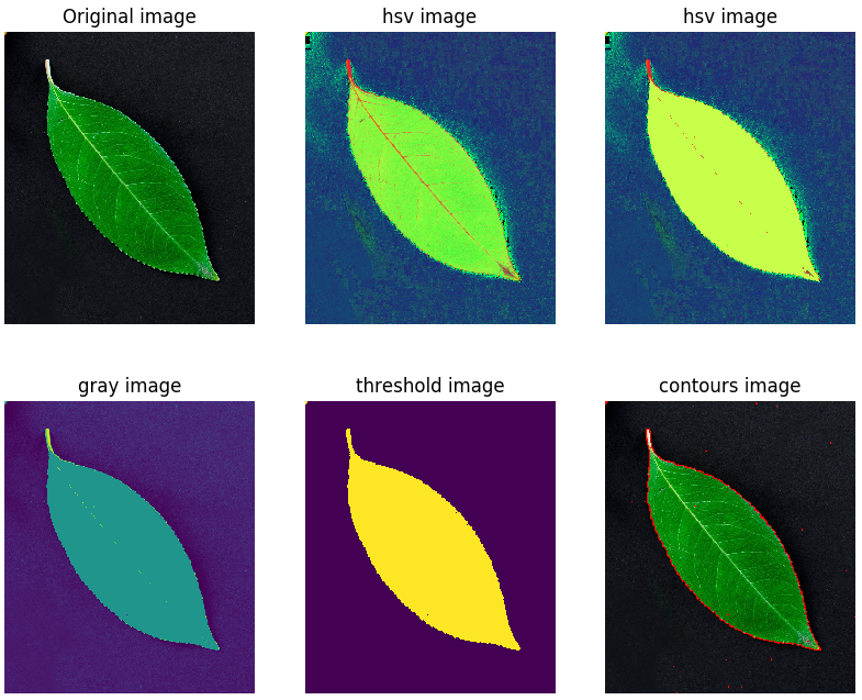
图7 - 处理过程与结果.
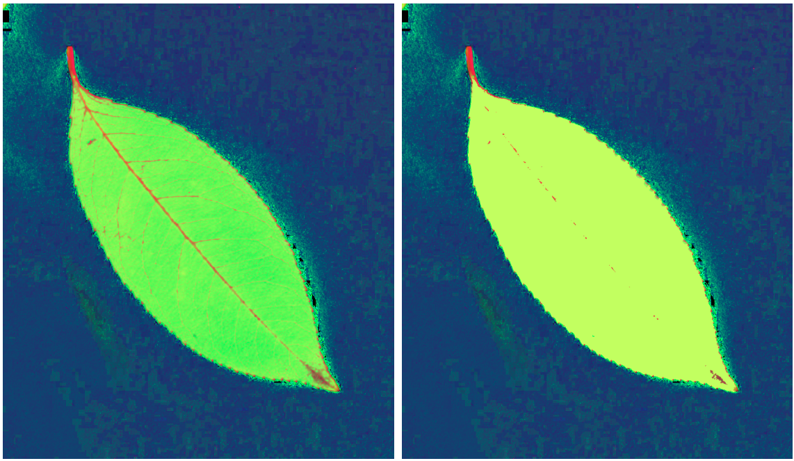
图8 - 左图:转换为HSV后的图像. 右图:应用 mask 后的图像(颜色统一)
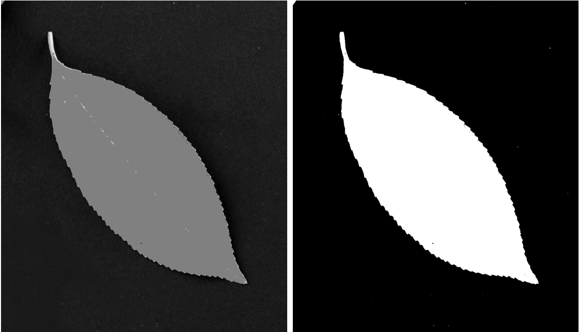
图9 - 左图:从HSV转换为灰色后的图像. 右图:阈值化的图像
由于背景中似乎也存在不规则性,可以使用这种方法获得最大的轮廓,最大的轮廓当然是叶子.
可以得到轮廓数组中叶子轮廓的索引,从中得到叶子的面积和中心.
轮廓具有许多其他可以使用的特征,例如轮廓周长,凸包,边界矩形等等. 可以参考 tutorial_py_contour_feature.
#找到最大面积的轮廓
def findGreatesContour(contours):
    largest_area = 0
    largest_contour_index = -1
    i = 0
    total_contours = len(contours)
    while (i < total_contours):
        area = cv2.contourArea(contours[i])
        if (area > largest_area):
            largest_area = area
            largest_contour_index = i
        i += 1

    return largest_area, largest_contour_index

# to get the center of the contour
cnt = contours[13]
M = cv2.moments(cnt)
cX = int(M["m10"] / M["m00"])
cY = int(M["m01"] / M["m00"])
largest_area, largest_contour_index = findGreatesContour(contours)
print(largest_area)
print(largest_contour_index)
print(len(contours))
print(cX)
print(cY)
输出:
278456.5
14
37
893
165